Spatial Transcriptomic Analysis
spata-introduction-and-philosophy.RmdSPATA - SPAtial Transcriptomic Analysis - provides a toolkit of R-functions and interactive applications to enable and facilitate the analysis of spatial transcription data. This includes easy to use interfaces, straightforward R-functions to easily visualize your data as well as more sophisticated ones for more experienced R users. The tutorials you’ll find on this website will guide you through everything SPATA provides. For more detailed information of whatever part you are interested in run ?SPATA::function-name in your R console.
SPATA Philosophy
Several R-packages that specialize on the analysis and visualization of spatial transcriptomic data have been released ever since the first paper on this approach has been published. Though all these packages come along with their own strengths and weaknesses we found it consistently difficult to integrate our own ideas into their predefined workflows which eventually motivated us to create SPATA. While SPATA introduces it’s own new spatial analysis aspects - such as spatial trajectory modeling - as well as it provides established visualization tools - such as surface plotting - it actually considers itself to be a more general framework that allows for easy integration of individual ideas and features. By providing such a framework and at the same time easy to use, interactive applications, full insight into functions and approaches we hope to speak to as many enthusiastic researchers as possible irrespective of their R-programming skills. Straightforward object-converting functions allow to switch from SPATA to different platforms such as Seurat or Monocle (and vice versa) at any timepoint, making it easy to leverage and integrate the advantages of all packages.
SPATA Concept
Throughout all functions and applications SPATA implements the tidy-data-concept and draws it’s main power from the tidyverse. With respect to the integration of individual analysis concepts this means in particular that all data.frames in SPATA are oriented towards the tidy-data structure in which each row represents an observation and every column represents a variable (information) of that observation. A consistent output and a consistent terminology facilitates the application of individual ideas via powerful tidyverse- and tidymodelling functions.
Tidy SPATA data.frames
With respect to the analysis of spatial transcriptomic data every observation in a what we call the spata-data.frame represents one barcode-spot and the belonging variables (columns) represent additional information related to these spots.
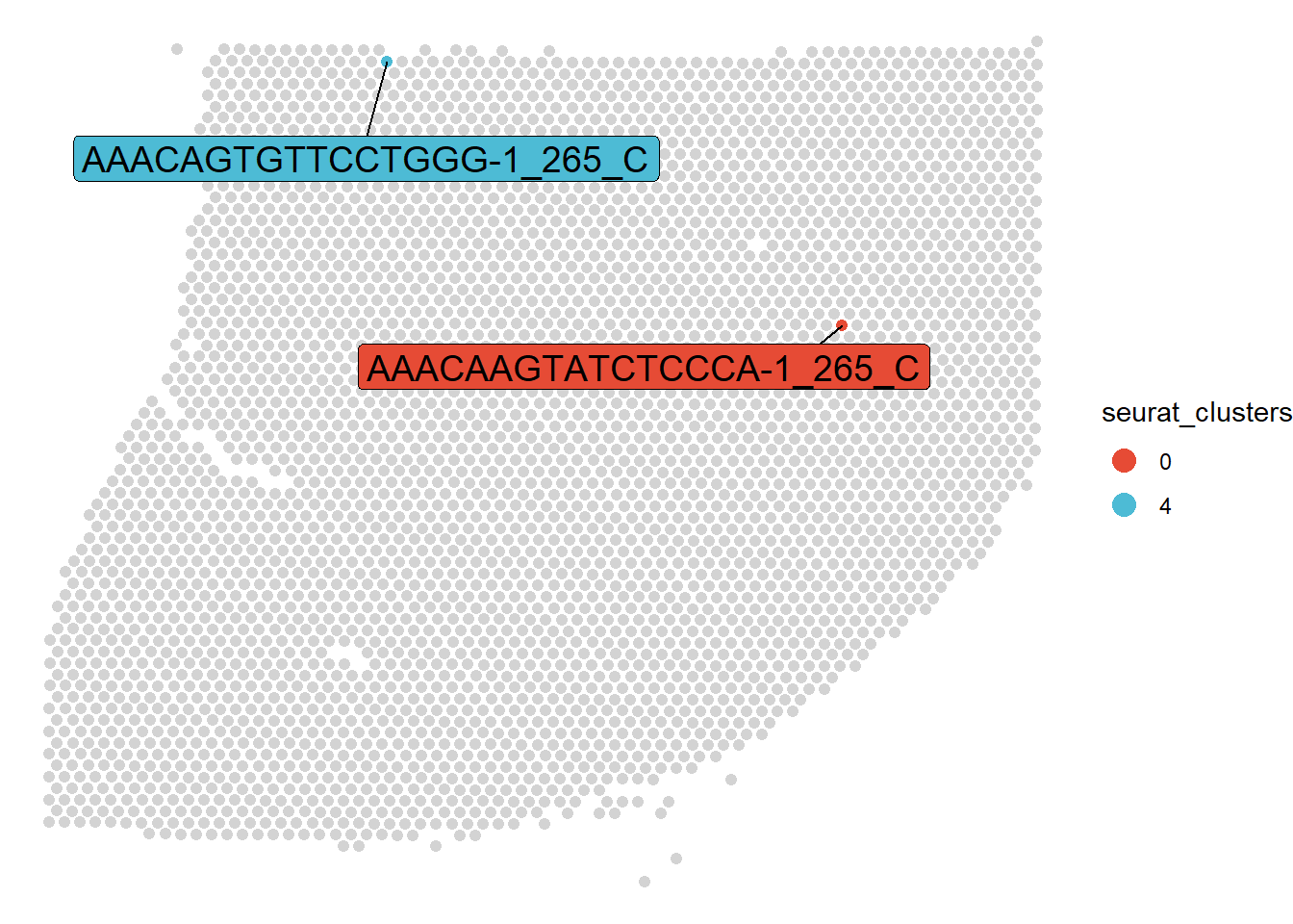
Figure 1. Examples of two barcode-spots
Apart from the barcode-sequence itself these information providing data-variables can be broadly divided into six classes:
Sample belonging refers to the sample a barcode-spot belongs to, which can be neglected if the spata-object contains only one sample.
Spatial information refers to every barcode’s position on the histology image via x- and y-coordinates.
Dimensional reduction refers to the every barcode’s position on UMAPs, TSNEs etc.
Gene expression refers to the expression levels every barcode’s-spot features for a particular gene. (e.g. ‘SLC35E2A’, ‘NADK’, ‘GFAP’)
Gene set expression refers to the expression values every barcode’s-spot features for a particular gene set. (e.g. ‘HALLMARK_HYPOXIA’)
Feature information refers to every additional information that has been calculated or simply added. (e.g. cluster belonging, imaging data, …)
Speaking of variables in subsequent tutorials, we refer to the latter three if not otherwise explained. The example data.frame below contains variables of all six types.
(To learn how to extract these data.frames from your spata-object see Extract, join & add data.)
Here every observation refers to one particular barcode spot. E.g. the first barcode-spot is labeled with the barcode ‘AAACAAGTATCTCCCA-1’, belongs to sample ‘265_C’, it’s coordinates on the spatial transcriptomic slide are 443.77 (x) and 373.901 (y). The clustering-algorithm has assigned it to cluster ‘0’, the gene expression level of this barcode-spot for gene SLC35E2A is 0.00 etc.
Informative variables vs. key variables
Features or gene- and gene-set expression usually vary (at least slightly) across barcode-spots but they are rarely unique across all of them. Barcode-spot’s barcode-sequences as well as their individual combination of x- and y-coordinates are always unique and we shall refer to these three variables from now on as key-variables in contrast to informative variables.
The fact that barcodes and coordinates uniquely identify each barcode-spot might sound obvious and barely of interest to anybody at first sight. From a data science perspective however, it harbors an immense power as these key-variables allow to integrate a potentially infinite number of dimensions to your analysis with ease. While the barcode-sequences allow for the integration of thousands of gene- and gene-set expression levels the coordinates allow to integrate all kinds of data coming along along with coordinates such as imaging data, spatial cytof data etc.
Though spatial transriptomic experiments come along with a spatial dimension gene- and gene-set expression data still resembles data of any other sequencing technique in a way that methods for the one technique are applicable to the other. The excellent R-package Seurat leverages that and provides a variety of tools to integrate spatial and single-cell data. Apart from it’s own new visualization- and analysis tools SPATA attempts to allow for easy integration of all kinds of data that come along with coordinates. Moreover it allows you to subsequently integrate this data in your Seurat- as well as in your Monocle3-workflow with convenient object-transforming functions.