Segmentation & Clustering
spata-segmentation-and-clustering.RmdDiscrete (syn. categorical) variables divide a sample’s barcode-spots into experimental groups that can be compared against each other.
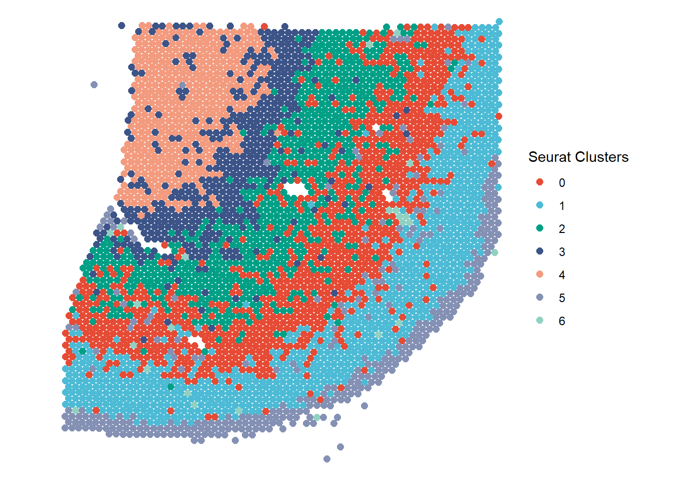
Figure 1.1 Example 1: Grouping the barcode-spots by clusters
Grouping of barcode-spots can be performed manually by determining spatial regions of interest and naming theme. (See below for more)

Figure 1.2 Example 2: Grouping the barcode-spots by manual, spatial segmentation
This tutorial guides you through the functions SPATA provides that allow for the gouping of barcode-spots.
Spatial segmentation
# load packages
library(SPATA)
library(magrittr)
library(ggplot2)

# load object
spata_obj <- loadSpataObject(input_path = "data/spata-obj-example-create-segm.RDS")
The spatial dimension of spatial transcriptomics invites to compare regions of interest against each other with respect to their gene expression or other features. The subpart-belonging of every barcode-spot is stored as an additional variable in the feature data. Assuming that you have not created any segments so far your feature data.frame will look like this:
Barcode spots that have not been assigned to a segment feature "" as their simply isn’t a segment to which they belong.
In order to to assign barcode-spots to a segment make use of the createSegmentation()-function. It opens a mini-shiny application in which you can determine the extent of every segment by determining the vertices of the polygon which determines the segment’s borders.
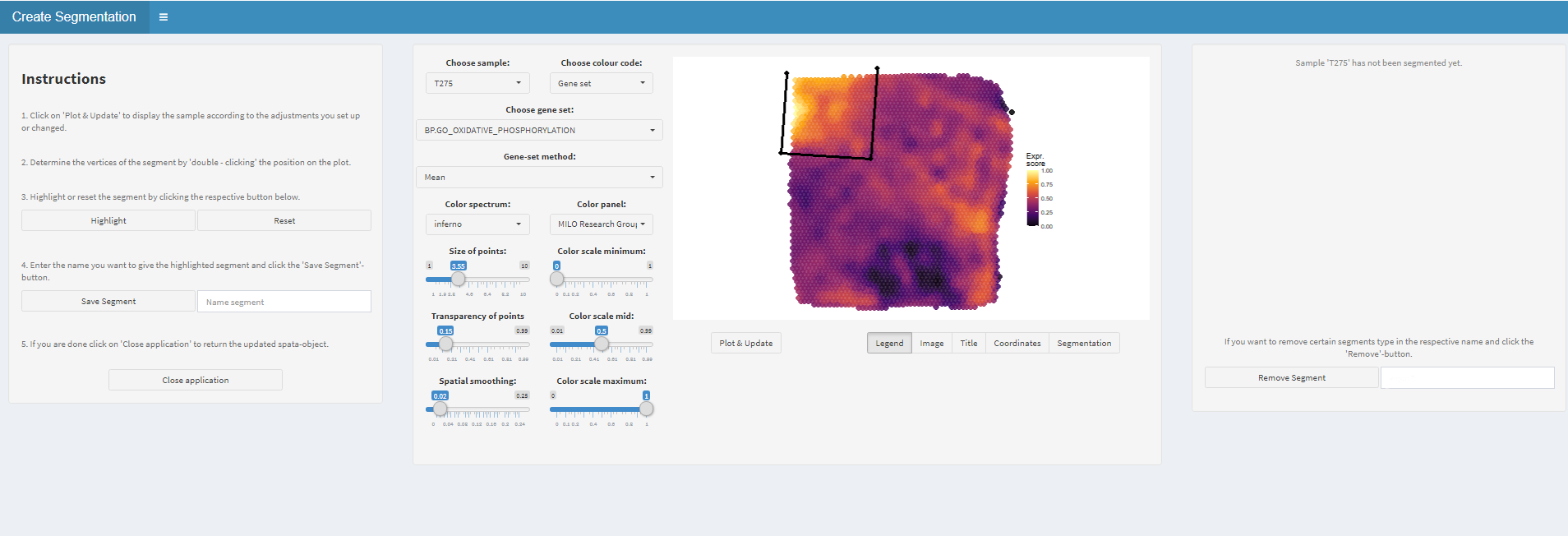
Figure 1.1) Easy interactive segmentation
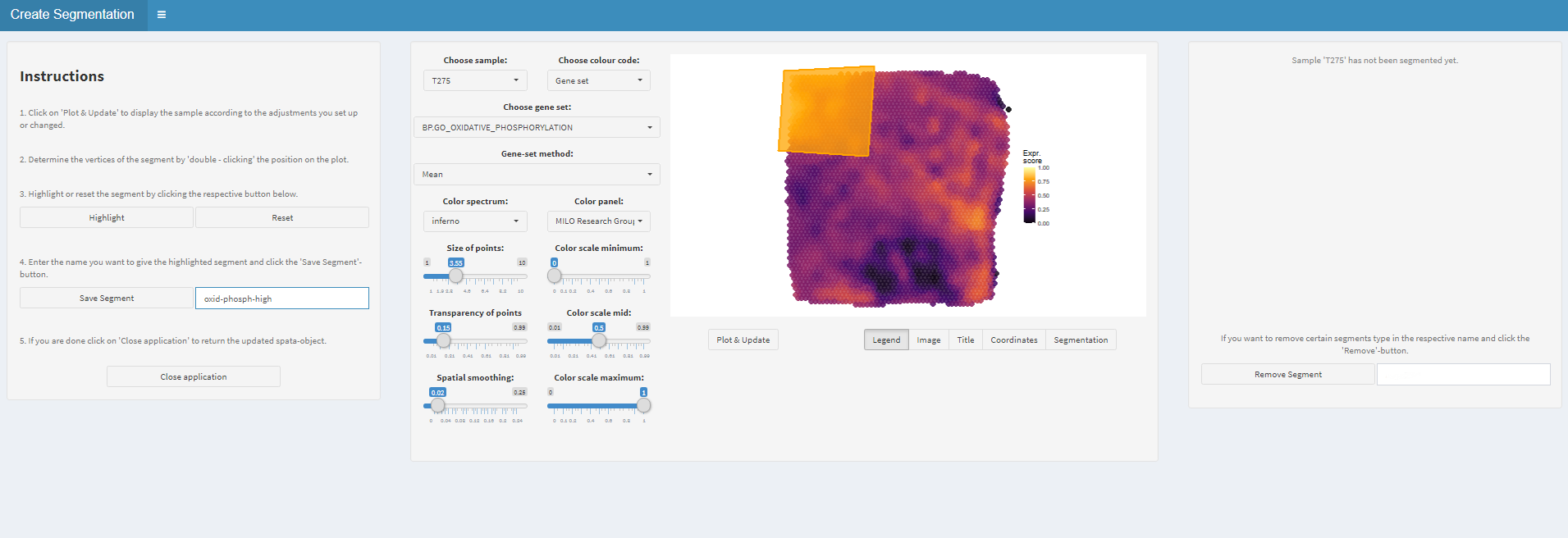
Figure 1.2) Highlight and save the segment
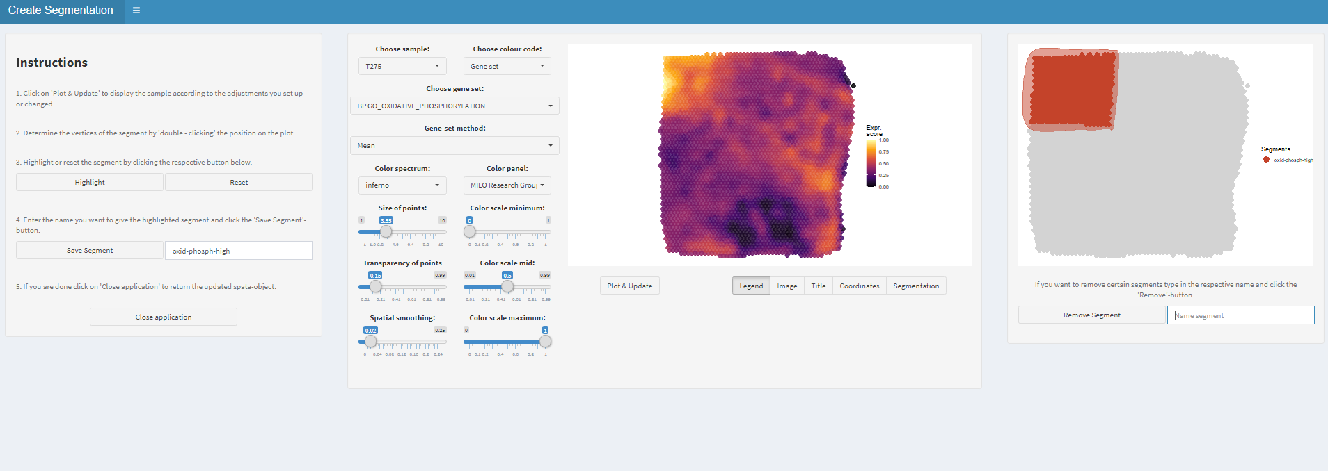
Figure 1.3) Save the segment and continue with the next area of interest
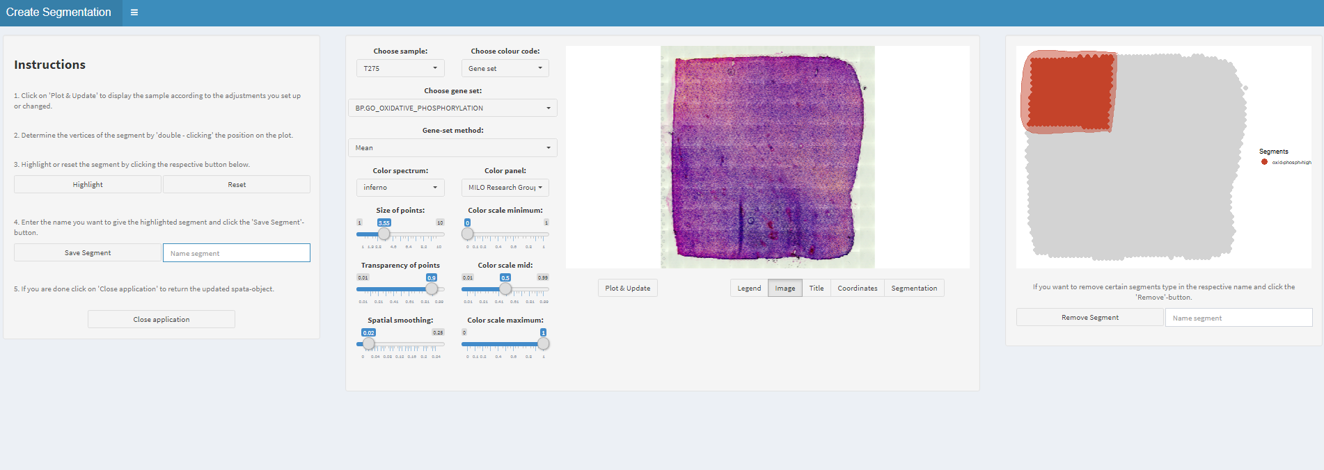
Figure 1.4) Set the transparency to max in order to see the histology
In order to visualize the current segmentation of your sample run plotSegmentation().
# display the current segmentation
plotSegmentation(spata_obj, pt_size = 2.5)
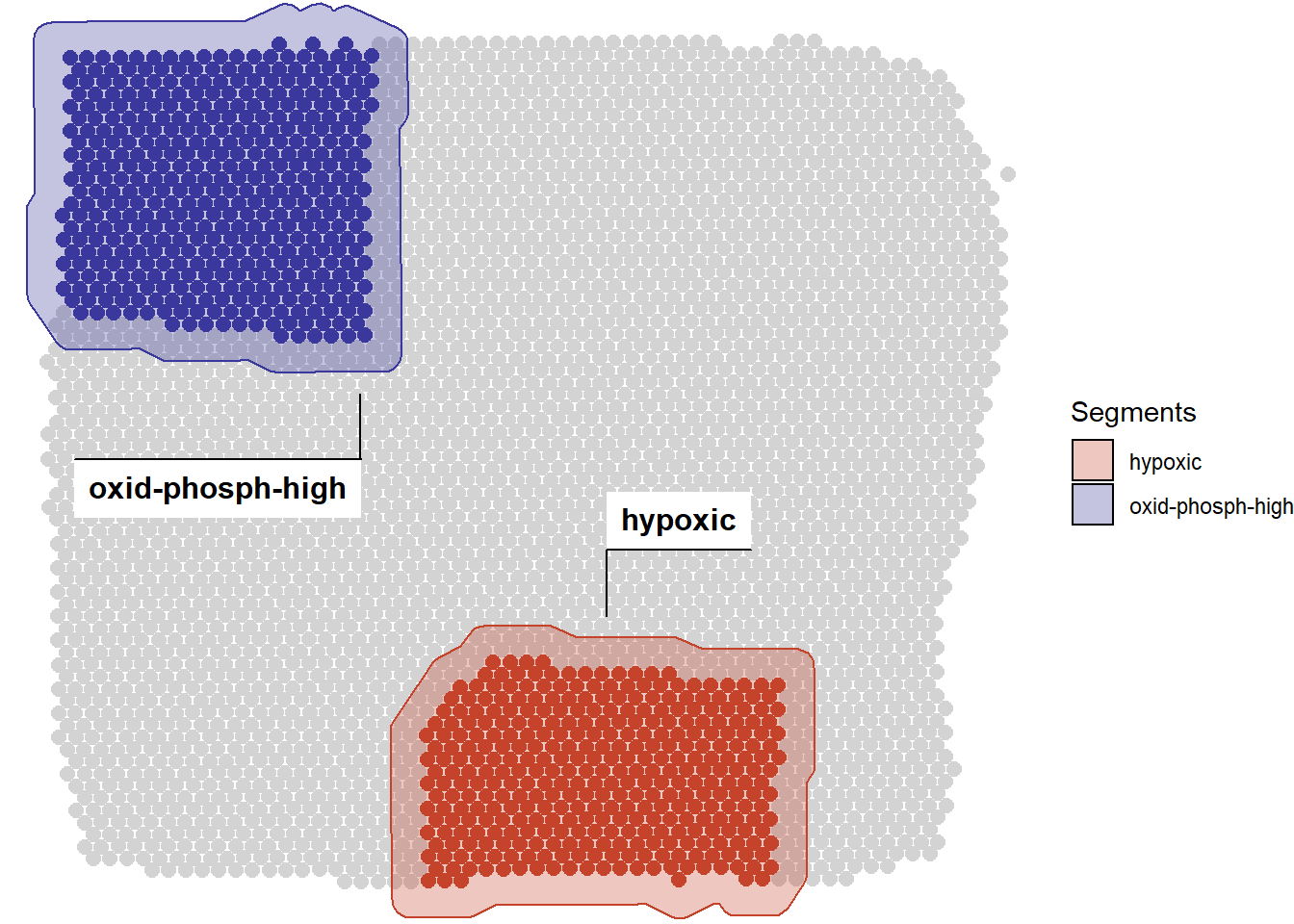
Figure 1.4) The current segmentation
The segment belonging is now a usable, discrete variable of your spata-object’s feature data, which can be used in SPATA as any other discrete feature and extracted in a tidy-data fashion as well.
getFeatureVariables(spata_obj, features = "segment", return = "data.frame")
If you need the barcodes of a segment’s barcode spots you can obtain them for example via getCoordinatesSegment().
getCoordinatesSegment(spata_obj, of_segment = "hypoxic")
Clustering
In transcriptomic analysis clustering divides barcode-spots into groups based on the similarity of their gene-expression profiles. There are several algorithms out there that can be used to divide your sample into subgroups. While initiateSpataObject_10X() integrates the clustering algorithm used by the Seurat-package there actually many more. As the use of clustering is highly depending on the biological question it makes sense to use several approaches.
Clustering with Monocle3
The package Monocle3 makes use of louvain- and leidenbase clustering with the cluster_cells()-function. This function takes several additional parameters that can be used to tweak the clustering-algorithm’s performance with respect to the properties of every individual sample. SPATA’s findMonocleClusters() is a wrapper around Monocle3’s clustering options. It iterates over the parameters you provide and returns a tidy spata data.frame containing each result as a seperate variable.
monocle_clusters <- findMonocleClusters(object = spata_obj,
                                        preprocess_method = "PCA",
                                        reduction_method = c("UMAP", "PCA", "tSNE"),
                                        cluster_method = c("leiden", "louvain"),
                                        k = 5,
                                        num_iter = 5)

# output
monocle_clusters
Use the helper function examineClusterResults() to quickly see all unique cluster names and to evaluate which clustering results come into question.
# output
examineClusterResults(data = monocle_clusters)
## $cluster_leiden_UMAP_k5
## [1] "Cluster 1" "Cluster 5" "Cluster 3" "Cluster 2" "Cluster 4" "Cluster 6"
## [7] "Cluster 7"
##
## $cluster_louvain_UMAP_k5
##  [1] "Cluster 29" "Cluster 43" "Cluster 16" "Cluster 27" "Cluster 37"
##  [6] "Cluster 14" "Cluster 36" "Cluster 38" "Cluster 17" "Cluster 8"
## [11] "Cluster 24" "Cluster 23" "Cluster 45" "Cluster 44" "Cluster 7"
## [16] "Cluster 40" "Cluster 34" "Cluster 1"  "Cluster 32" "Cluster 11"
## [21] "Cluster 21" "Cluster 6"  "Cluster 13" "Cluster 42" "Cluster 31"
## [26] "Cluster 41" "Cluster 12" "Cluster 20" "Cluster 26" "Cluster 2"
## [31] "Cluster 4"  "Cluster 28" "Cluster 25" "Cluster 18" "Cluster 46"
## [36] "Cluster 39" "Cluster 30" "Cluster 33" "Cluster 35" "Cluster 10"
## [41] "Cluster 15" "Cluster 9"  "Cluster 3"  "Cluster 19" "Cluster 5"
## [46] "Cluster 22"
##
## $cluster_leiden_PCA_k5
## [1] "Cluster 1" "Cluster 2"
##
## $cluster_louvain_PCA_k5
## [1] "Cluster 2" "Cluster 6" "Cluster 1" "Cluster 5" "Cluster 3" "Cluster 8"
## [7] "Cluster 9" "Cluster 7" "Cluster 4"
##
## $cluster_leiden_tSNE_k5
## [1] "Cluster 5" "Cluster 3" "Cluster 2" "Cluster 4" "Cluster 1" "Cluster 6"
## [7] "Cluster 7" "Cluster 8"
##
## $cluster_louvain_tSNE_k5
##  [1] "Cluster 10" "Cluster 28" "Cluster 6"  "Cluster 22" "Cluster 35"
##  [6] "Cluster 48" "Cluster 44" "Cluster 41" "Cluster 17" "Cluster 24"
## [11] "Cluster 25" "Cluster 12" "Cluster 23" "Cluster 39" "Cluster 19"
## [16] "Cluster 29" "Cluster 27" "Cluster 11" "Cluster 4"  "Cluster 33"
## [21] "Cluster 30" "Cluster 43" "Cluster 37" "Cluster 49" "Cluster 16"
## [26] "Cluster 40" "Cluster 21" "Cluster 13" "Cluster 3"  "Cluster 26"
## [31] "Cluster 46" "Cluster 2"  "Cluster 32" "Cluster 14" "Cluster 7"
## [36] "Cluster 38" "Cluster 47" "Cluster 9"  "Cluster 31" "Cluster 42"
## [41] "Cluster 15" "Cluster 20" "Cluster 18" "Cluster 8"  "Cluster 34"
## [46] "Cluster 5"  "Cluster 36" "Cluster 45" "Cluster 1"
It seems as if the results ‘cluster_leiden_UMAP_k5’, ‘cluster_leiden_tSNE_k5’, ’cluster_louvain_PCA_k5’ are the only ones that make sense to work with as the other three either result in way to many or way to less groups.
Via addFeatures() you can add all clustering results to your spata-object simultaneously, which makes them available for every SPATA-function. Each variable in monocle_clusters represents a possible option to assign barcodes to experimental groups. And since they are stored as individual variables they can be adduced, analyzed and visualized one by one.
# feature names before adding
getFeatureNames(spata_obj)
##           numeric           integer           numeric           numeric
##      "nCount_RNA"    "nFeature_RNA"      "percent.mt"      "percent.RB"
##            factor            factor         character
## "RNA_snn_res.0.8" "seurat_clusters"         "segment"
# add the cluster results spata_obj <- addFeatures(object = spata_obj, feature_names = c("cluster_leiden_UMAP_k5", "cluster_leiden_tSNE_k5","cluster_louvain_PCA_k5"), feature_df = monocle_clusters, key = "barcodes") # feature names afterwards getFeatureNames(spata_obj)
##                  numeric                  integer                  numeric
##             "nCount_RNA"           "nFeature_RNA"             "percent.mt"
##                  numeric                   factor                   factor
##             "percent.RB"        "RNA_snn_res.0.8"        "seurat_clusters"
##                character                character                character
##                "segment" "cluster_leiden_UMAP_k5" "cluster_louvain_PCA_k5"
##                character
## "cluster_leiden_tSNE_k5"
Continue by visualizing your results or by investigating their properties (e.g. differentially expressed genes).
plotSurface(object = spata_obj,
            color_to = "cluster_leiden_UMAP_k5",
            pt_size = 2.1,
            pt_clrp = "aaas") +
  labs(color = "Leiden UMAP")
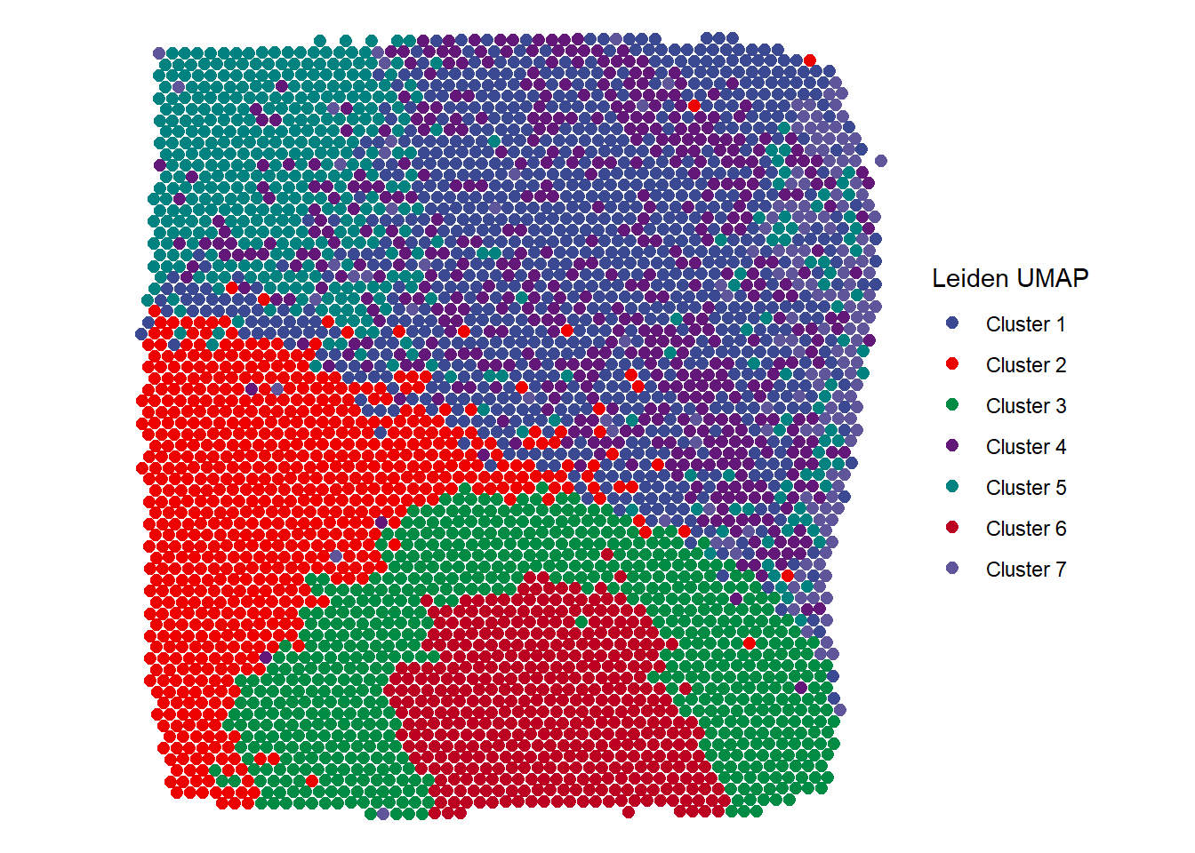
Figure 2.1 Easy visualization of different clustering results - Leiden UMAP
plotSurface(object = spata_obj,
            color_to = "cluster_leiden_tSNE_k5",
            pt_size = 2.1,
            pt_clrp = "jco") +
  labs(color = "Leiden tSNE")
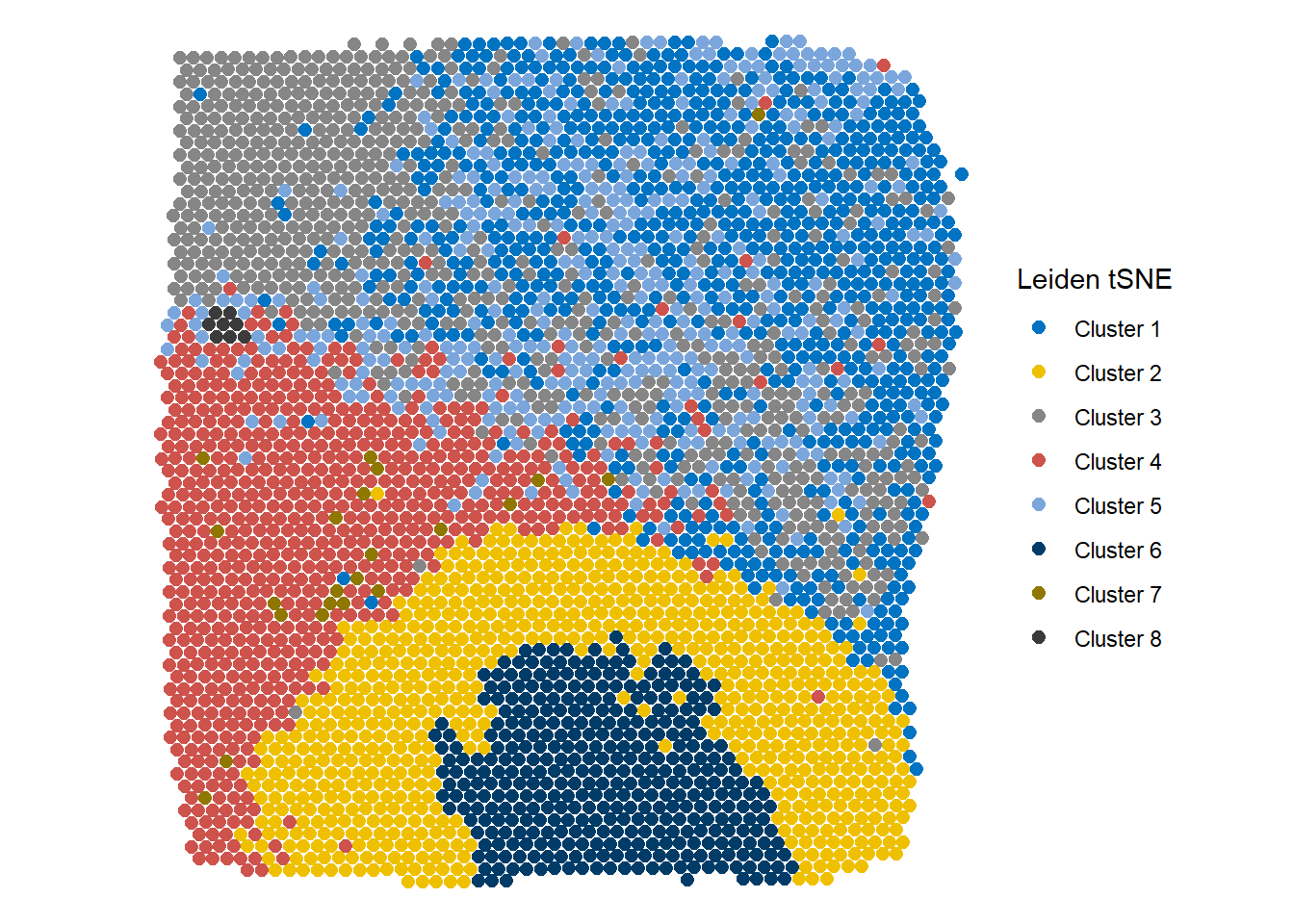
Figure 2.2 Easy visualization of different clustering results - Leiden tSNE
plotSurface(spata_obj,
            color_to = "cluster_louvain_PCA_k5",
            pt_size = 2.1,
            pt_clrp = "nejm") +
  labs(color = "Louvain PCA")
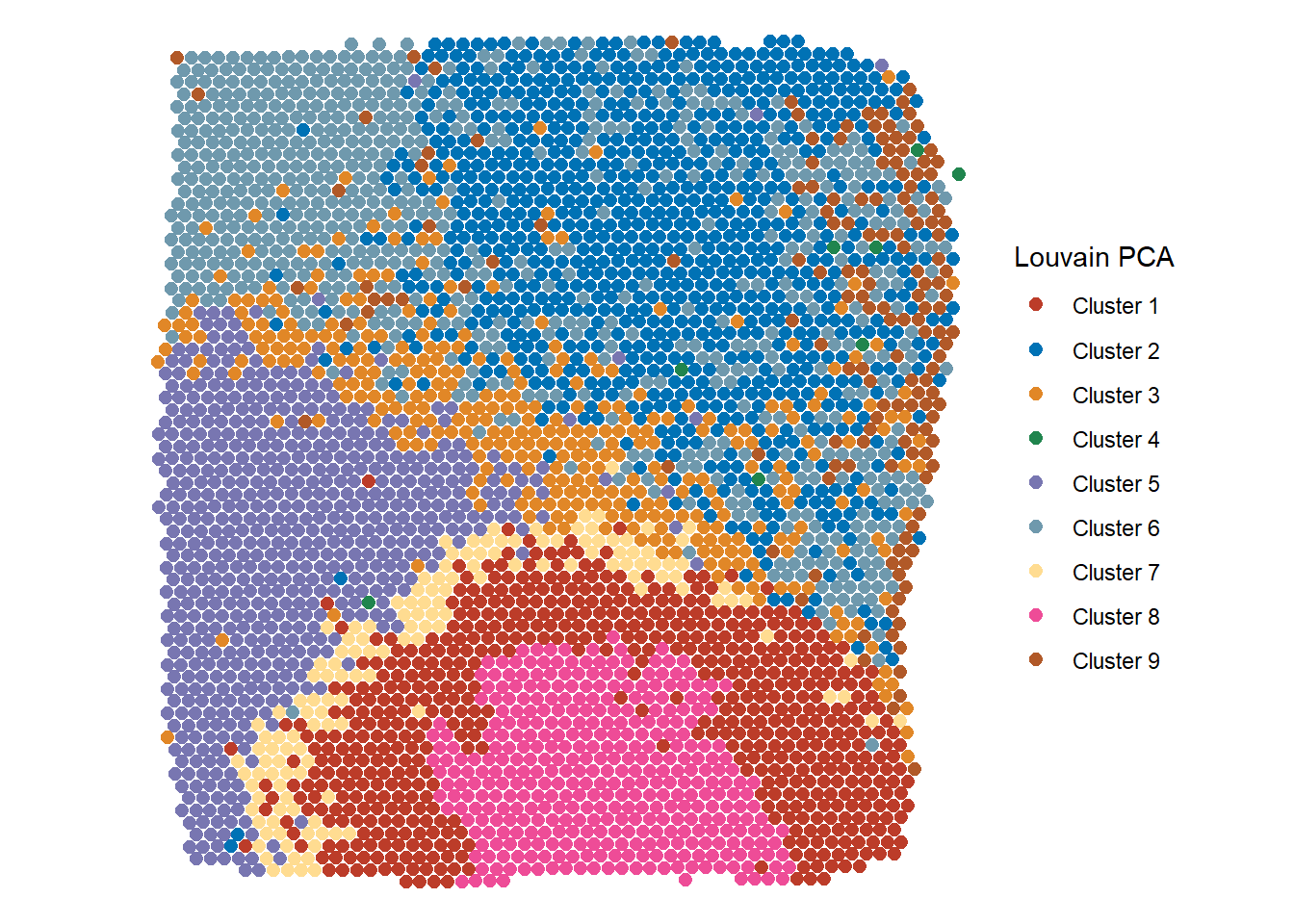
Figure 2.3 Easy visualization of different clustering results - Louvain PCA