Spatial trajectory analysis

With spatial trajectory analysis SPATA introduces a new approach to find, analyze and visualize differently expressed genes and gene-sets in a spatial context. While the classic differential gene expression analyzes this differences between experimental groups as a whole it neglects changes of expression levels that can only be seen while maintaining the spatial dimensions. Spatial trajectories allow to answer questions that include such a spatial component. E.g.:

1. In how far do expression levels change the more we move towards a region of interest?
2. Which genes follow the same pattern along these paths?

The spatial trajectory tools provided in SPATA enable new ways of visualization as well as new possibilities to screen for genes, gene-sets and patterns of interest.

# load package
library(SPATA)
library(magrittr)
library(ggplot2)
library(patchwork)

# load spata-object 
spata_obj <- loadSpataObject(input_path = "data/spata-obj-trajectory-analysis-tumor-example.RDS")

Draw trajectories

Spatial trajectories of a sample in a given spata-object can be drawn interactively using the function createTrajectories()as shown in the example below. createTrajectories() opens a mini-shiny application. This app allows one the one hand to investigate the sample with regards to spatial gene expression like plotSurfaceInteractive() does and on the other hand to draw trajectories through the areas of interest in four easy steps.

library(SPATA)

# open interactive application
spata_obj <- createTrajectories(object = spata_obj)

1. Drawing

Draw the trajectory interactively by clicking on the locations where you want the start and endpoints to be. If you click more than two times the trajectory is divided into sub-trajectory parts which will be displayed by subsequent plotting functions. Hence, it makes sense to stop everytime where you would expect a change as this will be highlighted by the transition from part to the subsequent one.

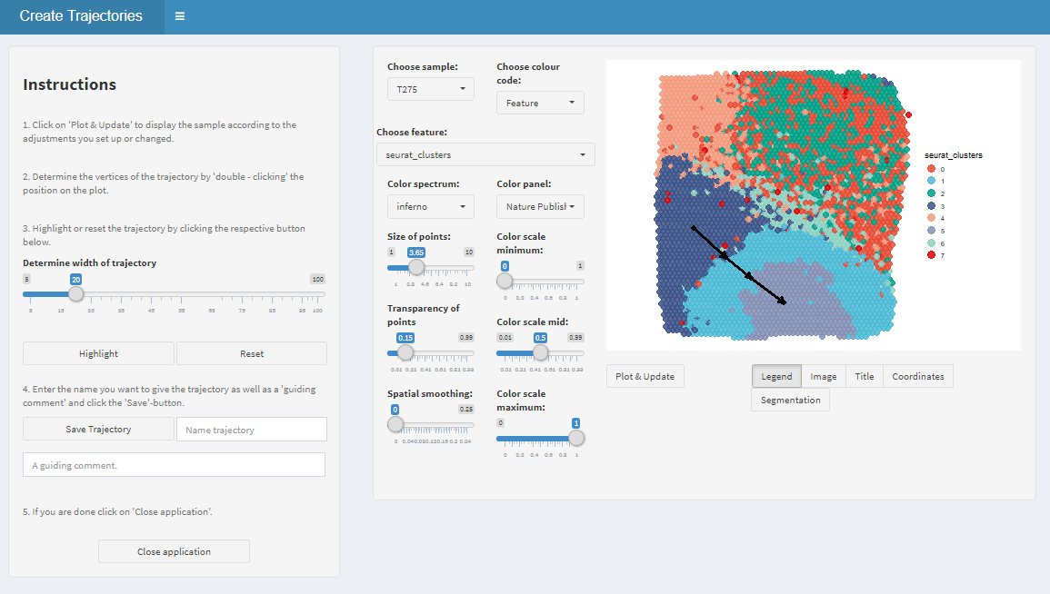
Figure 1.1. Interactive trajectory drawing

2. Highlighting

If start- and end-points are set adjust the trajectory width to and click on ‘Highlight’.

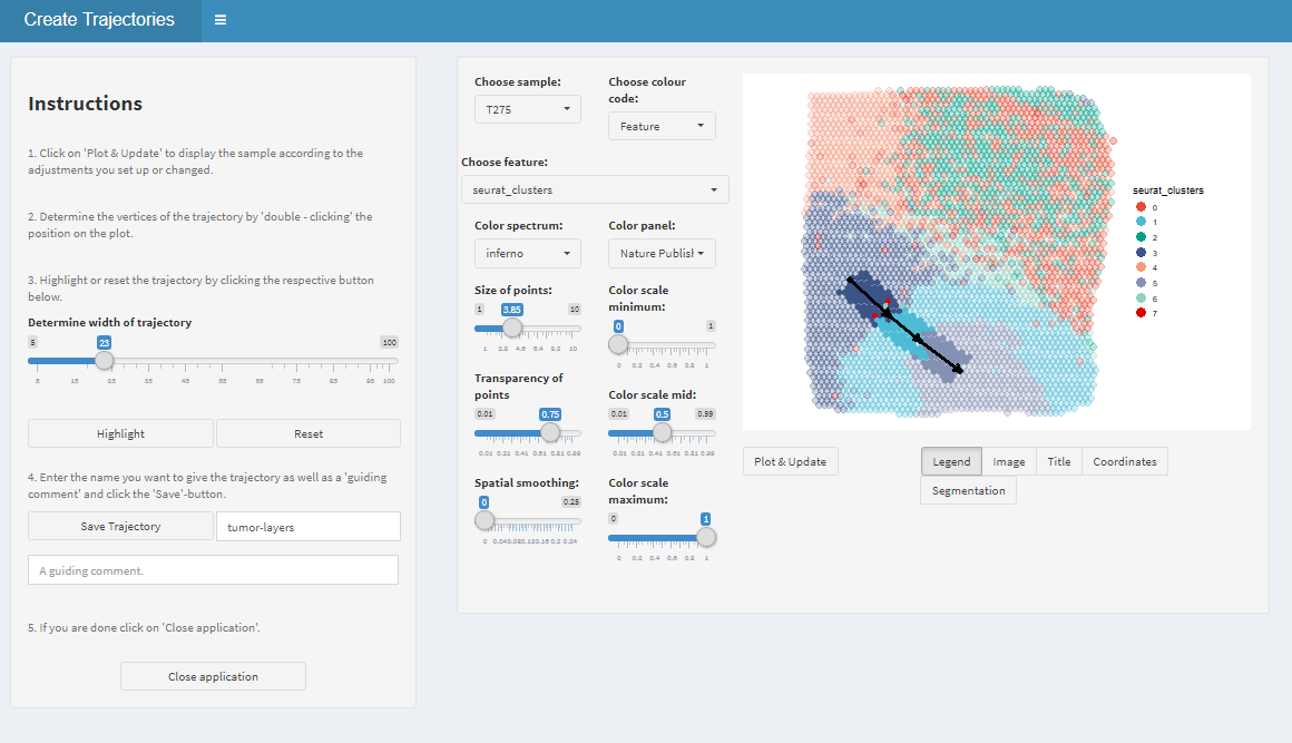
Figure 1.2. Highlight the trajectory

3. Naming

If you are satisfied with your trajectory enter a valid trajectory name and - if you want - a comment.

4. Saving

Click on ‘Save’ and on ‘Close application’ in order to return the updated spata-object.

Trajectories are stored inside the object itself. Therefore createTrajectories() returns an updated version of the object that was specified as the function’s input now containing the additional trajectories.

To obtain all trajectory names that have been drawn and saved in your spata-object use getTrajectoryNames(). Depending on the number of samples specified it returns a character vector or a list of such.

# get trajectory names 
getTrajectoryNames(object = spata_obj)

## [1] "tumor-layers"

Visualize trajectories

In order to visualize specific trajectories make use of plotTrajectory().

plotTrajectory(object = spata_obj,
               trajectory_name = "tumor-layers",
               color_to = "seurat_clusters",
               pt_size = 1.7,
               pt_clrp = "npg",
               display_image = FALSE) +
  theme(legend.position = "top") +

plotTrajectory(object = spata_obj,
               trajectory_name = "tumor-layers",
               color_to = "pseudotime",
               pt_size = 1.7,
               smooth = TRUE,
               smooth_span = 0.0125,
               display_image = FALSE) +
  theme(legend.position = "top")

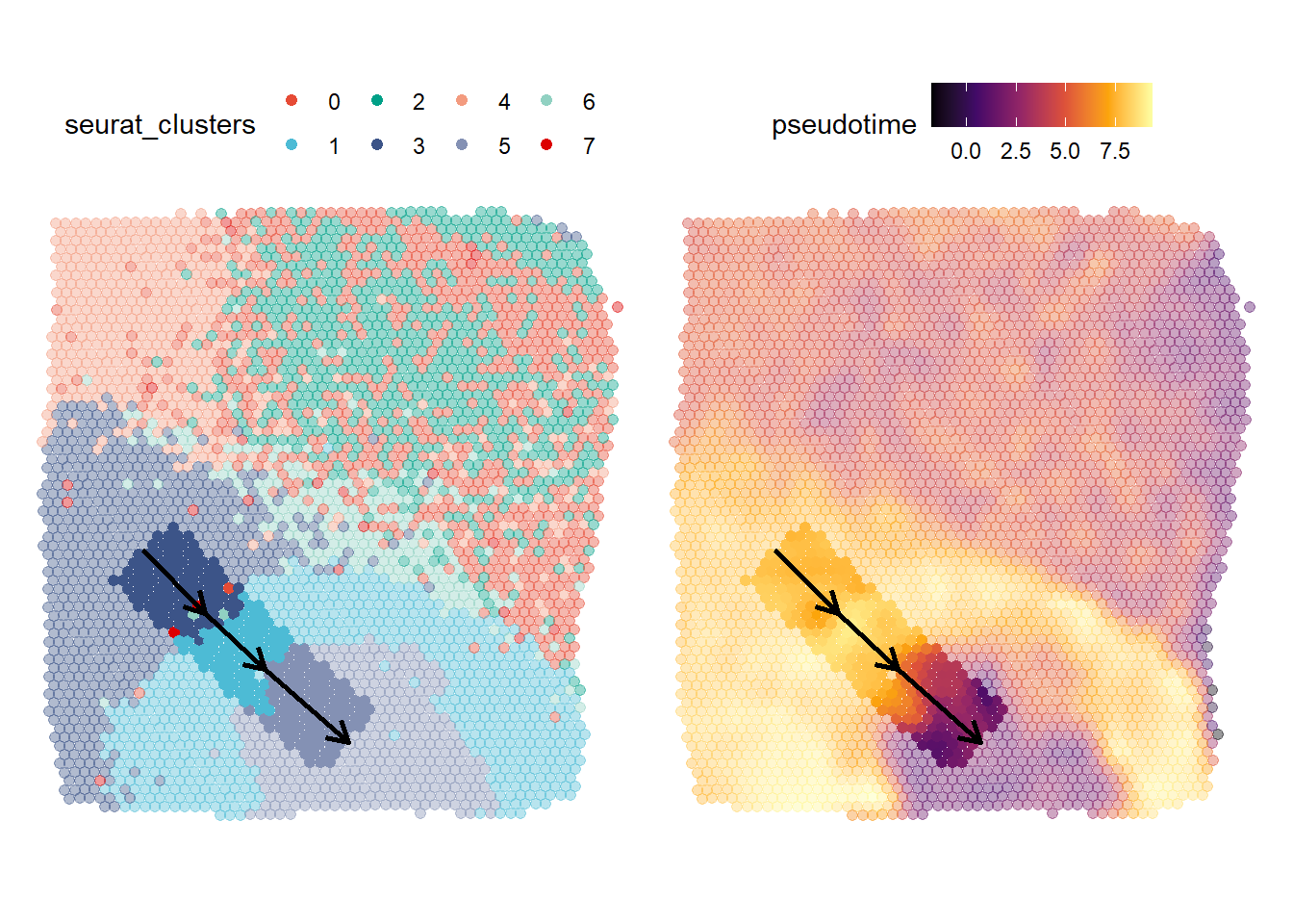
Figure 2.1. Surface related visualization of the trajectory

Visualize trajectory trends

Trajectory trends via lineplots

To display the trend of certain variables along a trajectory via lineplots use one of the following three functions:

• plotTrajectoryFeatures()
• plotTrajectoryGeneSets()
• plotTrajectoryGenes()

A call to one of those three functions will return a smoothed lineplot where the direction of the trajectory is mapped onto the x-axis and the values of the chosen aspects are mapped onto the y-axis. All functions follow the same concept and share the majority of their arguments. Still, they feature slight differences given the nature of their aspects to display.

The following three arguments have to be set in order to specify the trajectory that is to be analyzed:

• object
• trajectory_name
• of_sample (if more than one sample exists in the object, else it can be neglected)

The way values are smoothed and displayed can be manipulated via:

• smooth_method
• smooth_span
• smooth_se

Features along trajectories

Specify the features of interest via the argument features. Note that the function will compute the mean of all points on the axis orthogonal to the trajectory’s direction. As only numeric variables allow for such computation displaying the trend of categorical variables (e.g. cluster) is not possible via lineplots.

plotTrajectoryFeatures(object = spata_obj,
                       trajectory_name = "tumor-layers",
                       features = "pseudotime",
                       smooth_method = "loess",
                       smooth_span = 0.2,
                       smooth_se = TRUE)

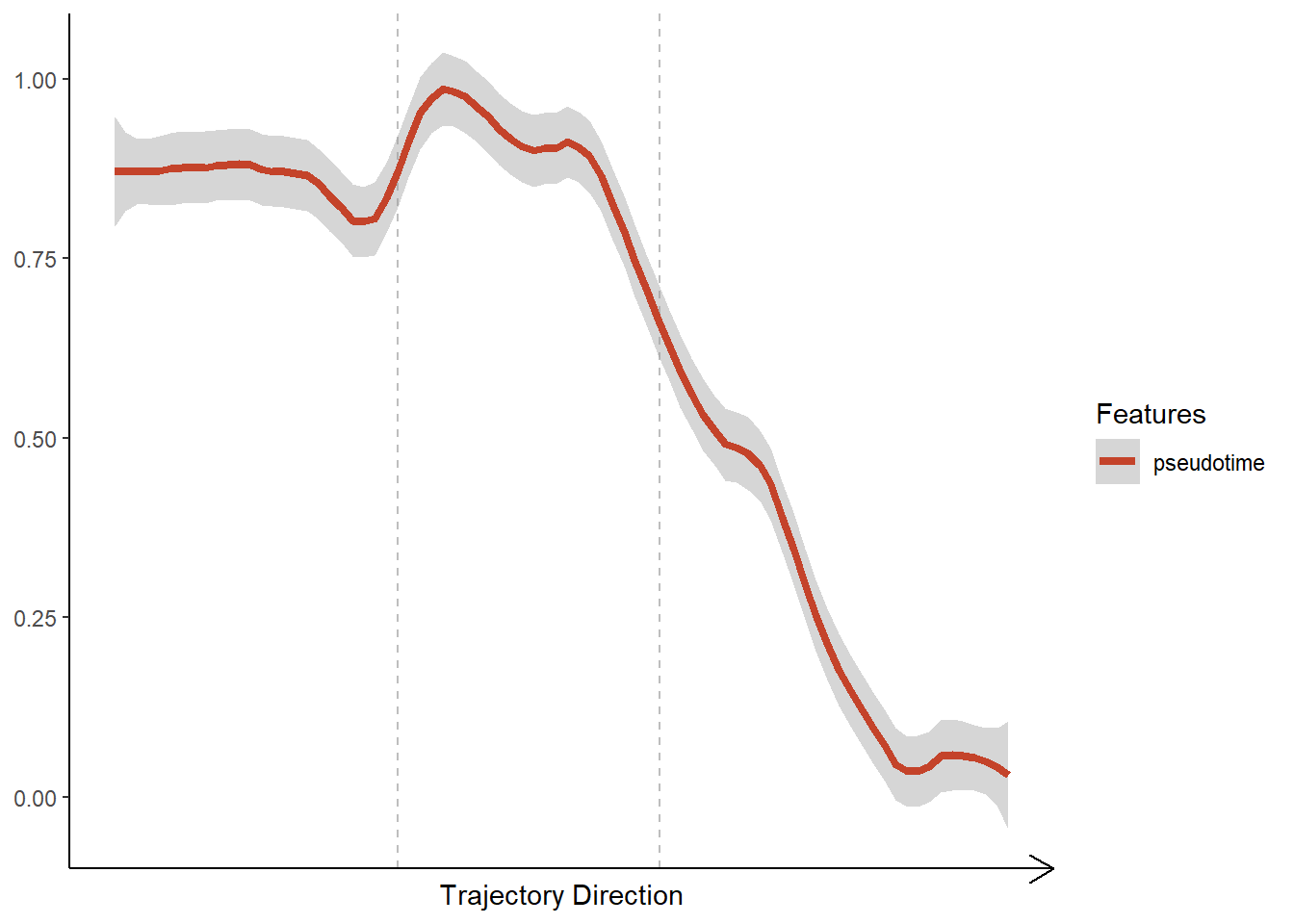
Figure 3.1. Visualization of ontinuous features along a trajectory

In order to plot discrete features use plotTrajectoryFeaturesDiscrete().

plotTrajectoryFeaturesDiscrete(object = spata_obj,
                               trajectory_name = "tumor-layers",
                               discrete_feature = "seurat_clusters",
                               clrp = "npg",
                               display_trajectory_parts = FALSE)

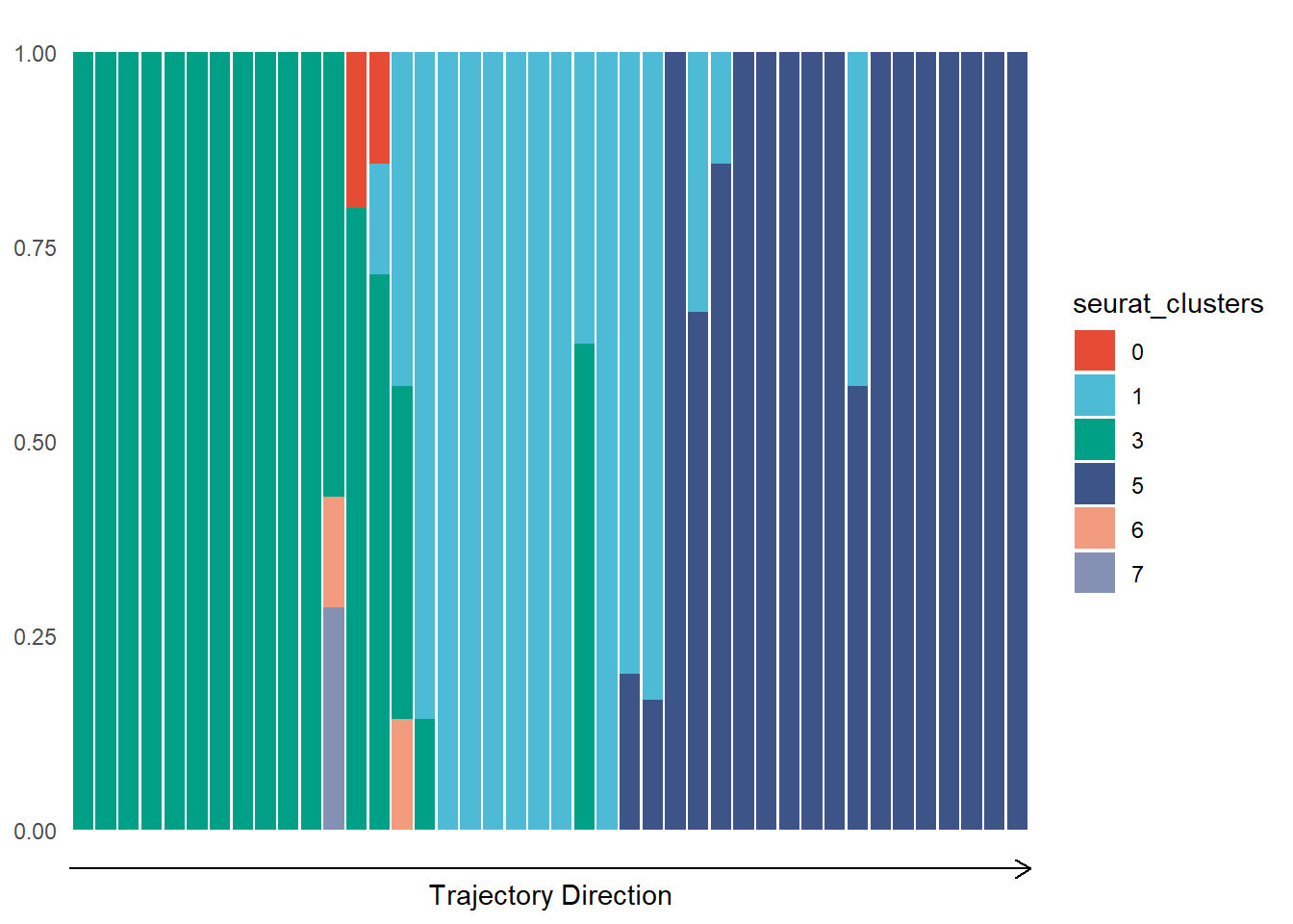
Figure 3.2. Visualization of discrete features along a trajectory

Genes and gene-sets along trajectories

Specify the genes or gene-sets of interest by using the respective functions and arguments.

# gene-set names
genes_of_interest <- c("CALM1", "VIM", "GFAP")

# plot lineplot
plotTrajectoryGenes(object = spata_obj,
                    trajectory_name = "tumor-layers",
                    genes = genes_of_interest,
                    smooth_span = 0.2,
                    smooth_se = TRUE)

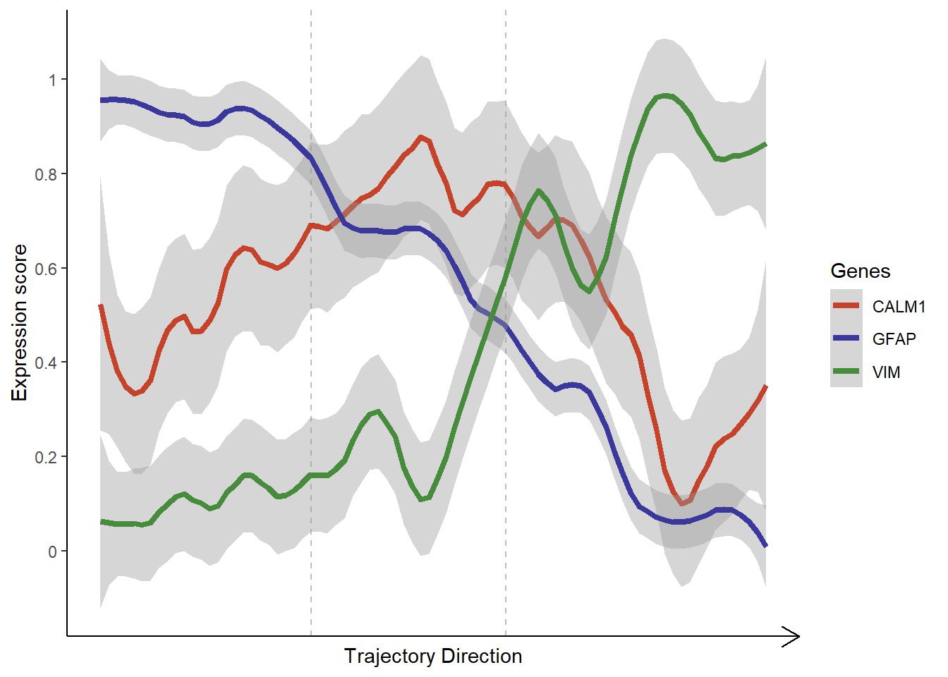
Figure 3.3. Visualization of gene expression along a trajectory

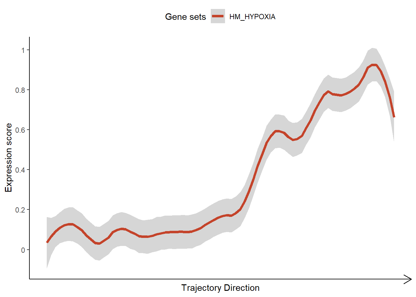
plotTrajectoryGeneSets(
  object = spata_obj,
  trajectory_name = "tumor-layers",
  gene_sets = "HM_HYPOXIA",
  display_trajectory_parts = FALSE) + # results in missing vertical lines 
  ggplot2::theme(legend.position = "top")

Analyze & model trajectories

To find variables that follow a certain trend along the trajectory of interest use assessTrajectoryTrends(). It fits the trajectory-trends of all specified variables to a variety of patterns and assesses their fit by calculating the area under the curve of the residuals.

all_genes <- getGenes(spata_obj)
all_gene_sets <- getGeneSets(spata_obj)

# obtain an assessed trajectory data.frame for all genes
atdf_gs <- assessTrajectoryTrends(object = spata_obj,
                                  trajectory_name = "tumor-layers",
                                  variables = all_genes)

# obtain an assessed trajectory data.frame for all gene-sets
atdf_gene_sets <- assessTrajectoryTrends(object = spata_obj,
                                         trajectory_name = "tumor-layers",
                                         variables = all_gene-sets)

# output example
atdf_gs

The resulting data.frame contains the evaluation of all fits for all provided variables. plotTrajectoryFit() visualizes the fitting results for a particular variable.

# compare the trend of a variable to different models
plotTrajectoryFit(object = spata_obj,
                  trajectory_name = "tumor-layers",
                  variable = "GFAP",
                  display_residuals = TRUE) +
  ggplot2::theme(legend.position = "top")

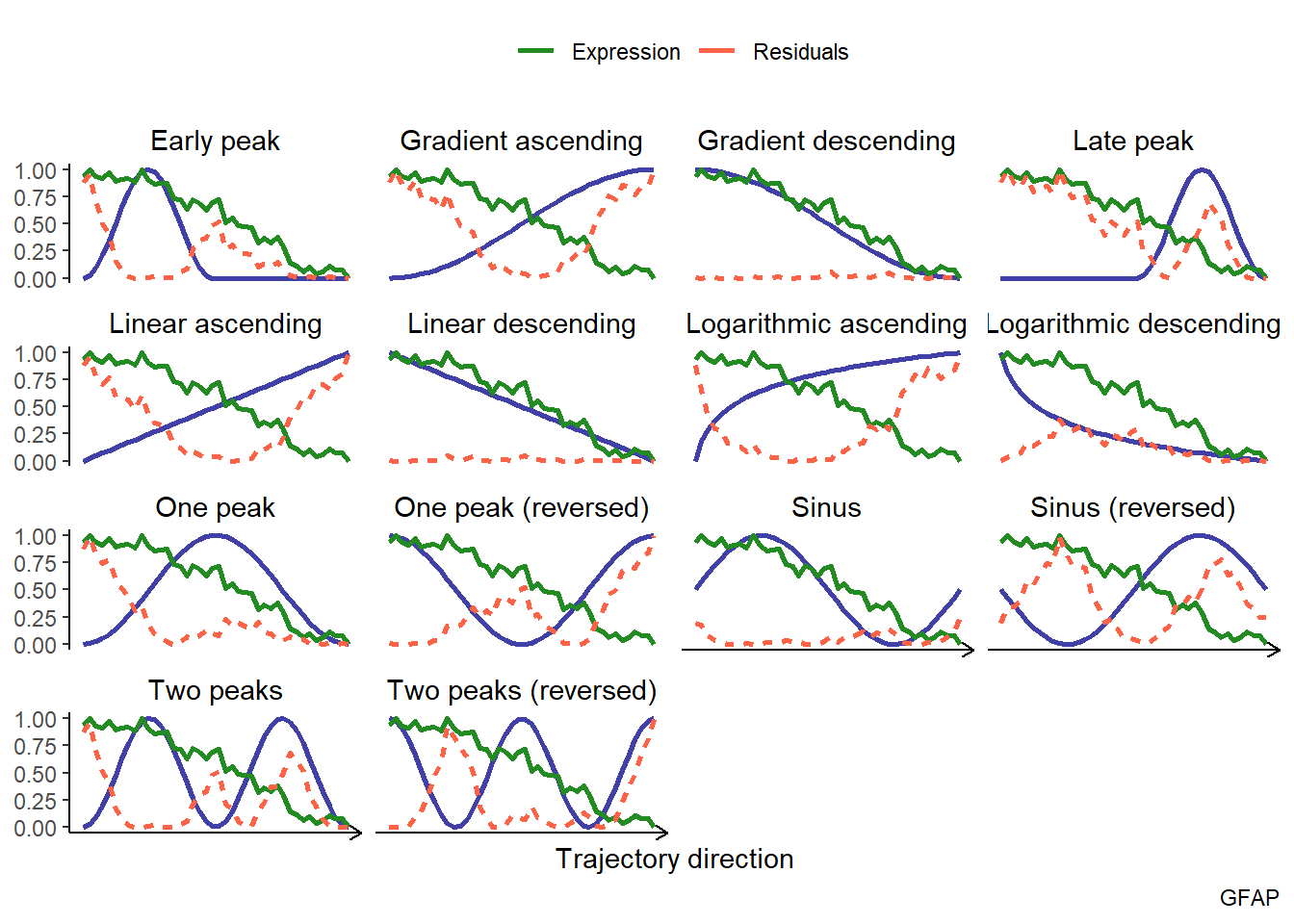
Figure 4.1. Visulization of the fitting results

To get a summary of your trajectory assessment use examineTrajectoryAssessment() which displays the distribution of all areas under the curve measured. Use filterTrend() or a combination of dplyr::filter()and dplyr::pull() on your assessed trajectory data.frame in order to extract the variables following a specific trend to a certain quality-degree.

# example 1: extract all variables that follow the linear descending trend while moving towards the hypoxic area (See Figure 2.1)
# with an auc-evaluation equal to or lower than 2
descending_gene_sets <-
  filterTrends(atdf = atdf_gene_sets,
               limit = 2,
               trends = c("Linear descending"),
               variables_only = FALSE) # return a data.frame

descending_gene_sets

# example 2: extract variables that featured a peak along the trajectory 
# with auc-evaluation equal to or lower than 4
peaking_genes <- filterTrends(atdf = atdf_gs,
                              limit = 4,
                              trends = c("Early peak", "Late peak", "One peak"),
                              variables_only = TRUE) # return a vector of variables

head(peaking_genes)

## [1] "CKB"    "METRN"  "TMSB4X" "LPL"    "CALM1"  "ITGA3"

Trajectory trends via heatmaps

Displaying the expression trends of too many variables in a lineplot gets unclear quite rapidly. In order to deal with several variables use plotTrajectoryHeatmap(). While the trajectory’s directory is still displayed from left to right the dynamic of the gene-sets’ expression values is now displayed by the gradual change of a row’s color instead of a line’s slope in a lineplot. The advantage of using heatmaps to display dynamic expression changes along trajectories becomes obvious when the number of variables to display rises.

descending_gene_sets <- dplyr::pull(descending_gene_sets, variables)

plotTrajectoryHeatmap(object = spata_obj,
                      trajectory_name = "tumor-layers",
                      variables = descending_gene_sets,
                      arrange_rows = "maxima",
                      show_row_names = FALSE, # gene set names are long...
                      split_columns = TRUE,
                      smooth_span = 0.5)

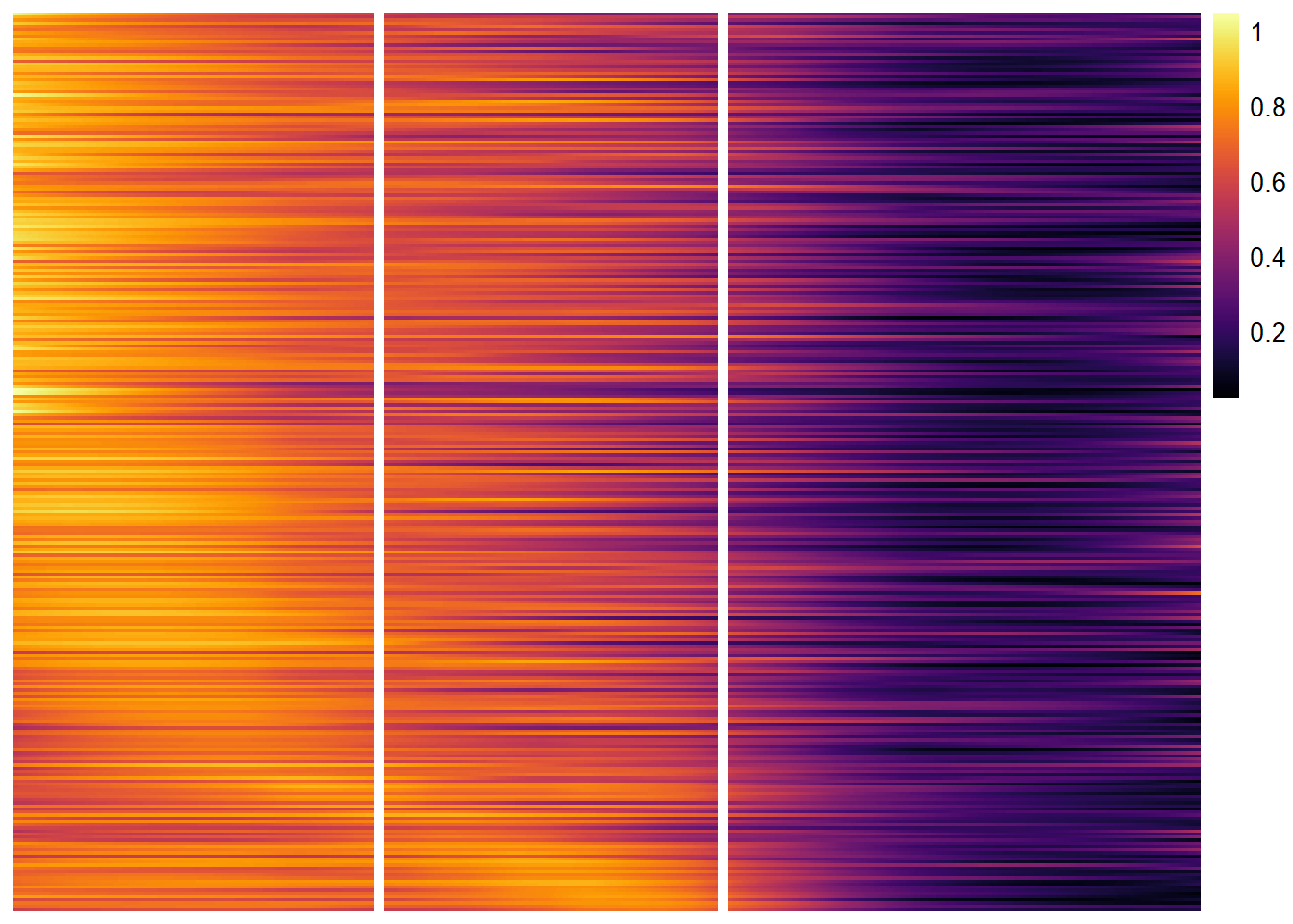
Figure 4.2) A heatmap displaying linear descending trends

plotTrajectoryHeatmap(object = spata_obj,
                      trajectory_name = "tumor-layers",
                      variables = peaking_genes,
                      arrange_rows = "maxima",
                      show_row_names = FALSE, # gene set names are long...
                      split_columns = TRUE, # splits the heatmap 
                      smooth_span = 0.5)

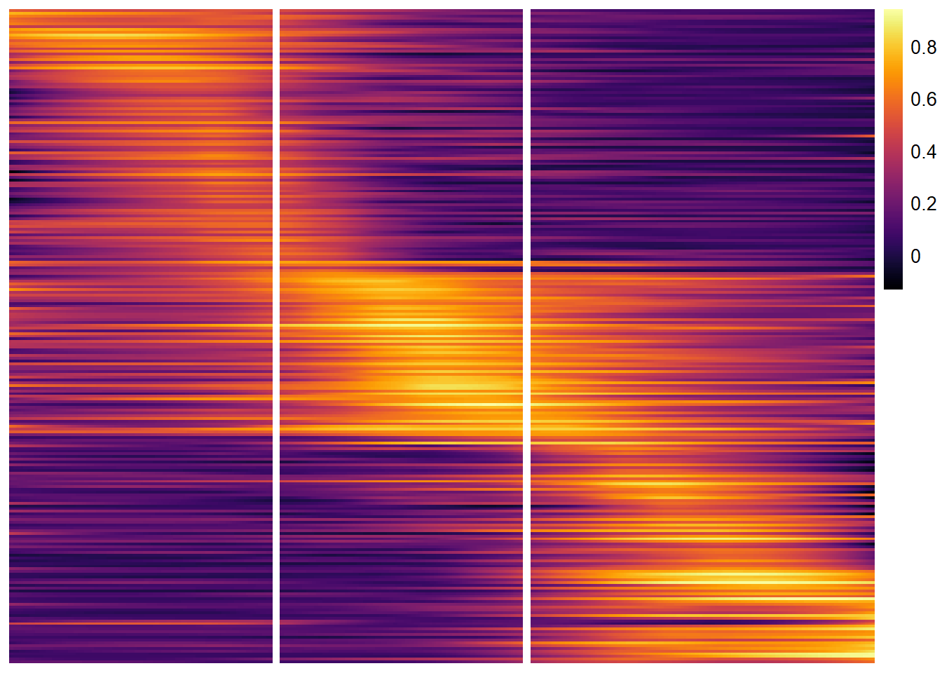
Figure 4.3. A heatmap displaying the gradual change of peaking genes