SPATA & other platforms
spata-compatibility.RmdApart from SPATA there have been published several packages that devote themself to the analysis of sequencing data. Two of them are Monocle3 and Seurat. This article demonstrates how to leverage SPATA’s compatibility.
Monocle3
The package monocle3 provides a variety of tools to analyze and visualize single-cell-sequencing data. Though spatial transcriptomic experiments do not reach the resolution of single-cell-sequencing yet you can leverage a variety of monocle3’s functions for your analysis and easily integrate the results back to your spata-object.
# load packages
library(SPATA)
library(magrittr)

library(tidyverse)
library(patchwork)

library(monocle3)

# load example of human brain cortex
spata_obj <- loadSpataObject(input_path = "data/spata-obj-monocle-cortex.RDS")
In order to work with the functions of monocle3 you need to compile it’s core object: the cell_data-set. You can do that with ease with compileCellDataSet(). It is a wrapper around all of monocle3’s pre processing functions, takes your spata-object of interest and creates a cell_data_set from it’s count matrix. Convenient argument input via named lists and defensive error handling via base::tryCatch() allow more experienced users to tweak the pre processing results. For the sake of simplicity we stick to the default options throughout this example.
# compile a cell-data-set
cortex_cds <- compileCellDataSet(object = spata_obj)
spata_plot <-
  plotSurface(spata_obj, color_to = "seurat_clusters", pt_clrp = "npg") +
      theme(legend.position = "bottom") +
      labs(color = "Seurat Clusters") +
      ggplot2::guides(color = ggplot2::guide_legend(override.aes = list(size = 4)))


# SPATAS compile functions pass the feature data to the compiled object which makes
# all features computed by yourself available, e.g. for monocle3::plot_cells()
monocle_plot <-
  plot_cells(cortex_cds, reduction_method = "UMAP", color_cells_by = "seurat_clusters") +
      scale_color_add_on(aes = "color", variable = "discrete", clrp = "npg") +
      theme(legend.position = "none")

# output 1 & 2
spata_plot

monocle_plot
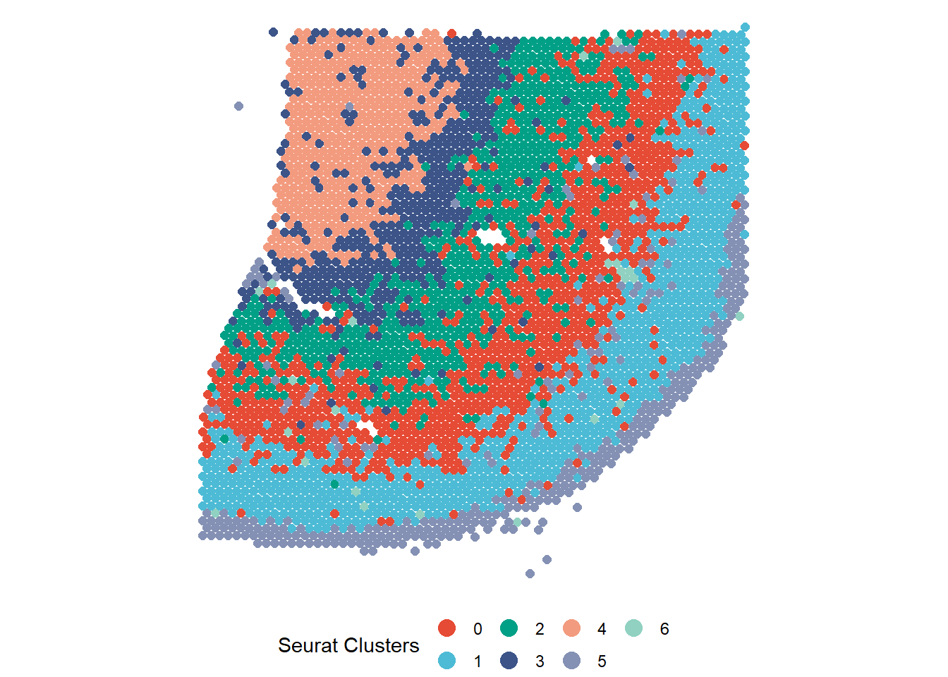
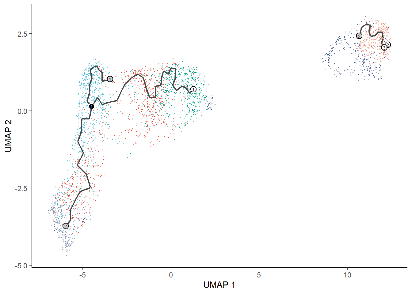
Figure 1 SPATA’s and monocle3’ basic plotting results
Example 1 - Pseudotime
If you haven’t done it already during cortex_cds’s compilation you can use moncle3::order_cells() to work with pseudotime - a measurement of how much progress cells have made through a process such as cell differentiation.
# the pseudotime values for all cells/barcode-spots are obtained via
pseudotime_vec <- pseudotime(cortex_cds)

# subset output
pseudotime_vec[1:10]
## AAACAAGTATCTCCCA-1_C265 AAACACCAATAACTGC-1_C265 AAACAGTGTTCCTGGG-1_C265
##            1.158532e+01            1.489730e-01            2.742735e-03
## AAACATTTCCCGGATT-1_C265 AAACCCGAACGAAATC-1_C265 AAACCGGAAATGTTAA-1_C265
##            4.136091e+00            1.021155e+01            7.852228e+00
## AAACCGGGTAGGTACC-1_C265 AAACCGTTCGTCCAGG-1_C265 AAACCTAAGCAGCCGG-1_C265
##            2.422186e+00            8.473789e-01            1.832179e-04
## AAACCTCATGAAGTTG-1_C265
##            1.815821e-04
The output of monocle3::pseudotime() is a named vector of numeric values where by the numeric value refers to a barcode-spot’s pseudotime value and the name to it’s sequence. We can easily join this information to our original spata-object with a little bit of data wrangling and the addFeature()-function.
# 1. convert to data.frame
pseudotime_df <- as.data.frame(pseudotime_vec)

# output
pseudotime_df
# 2. create a barcodes-key variable and rename the pseudotime variable
feature_df <-
  magrittr::set_colnames(x = pseudotime_df, value = "Pseudotime") %>%
  tibble::rownames_to_column(var = "barcodes")

# output
feature_df
# 3. add to spata-object via
spata_obj <- addFeatures(object = spata_obj,
                         feature_names = "Pseudotime",
                         feature_df = feature_df,
                         key_variable = "barcodes")
The feature Pseudotime is now a valid feature in our spata-object and thus accessible via all functions in SPATA that take numeric features as an input option.
# visualize pseudotime on the surface
plotSurface(spata_obj, color_to = "Pseudotime", smooth = TRUE, smooth_span = 0.02, pt_size = 2.2)
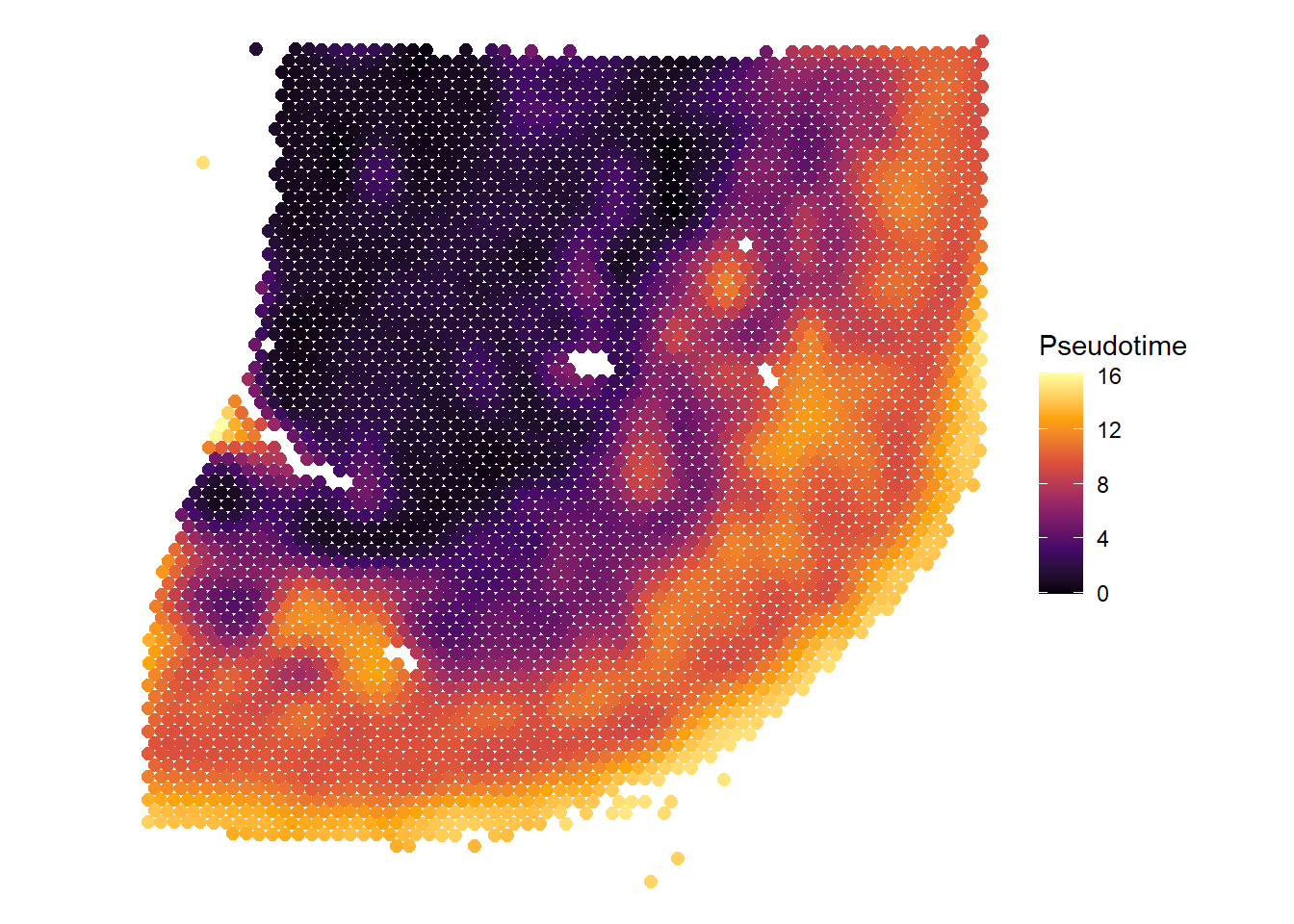
Figure 2 Visualizing monocle3-pseudotime results with SPATA
Example 2 - Clustering
The same concept can be applied to clustering-results. findMonocleClusters() is a convenient wrapper around the different clustering algorithms relies on. Alternatively one can extract the different clustering results from the cell_data_set created with compileCellDataSet() manually in order to add it to the spata-object one by one.
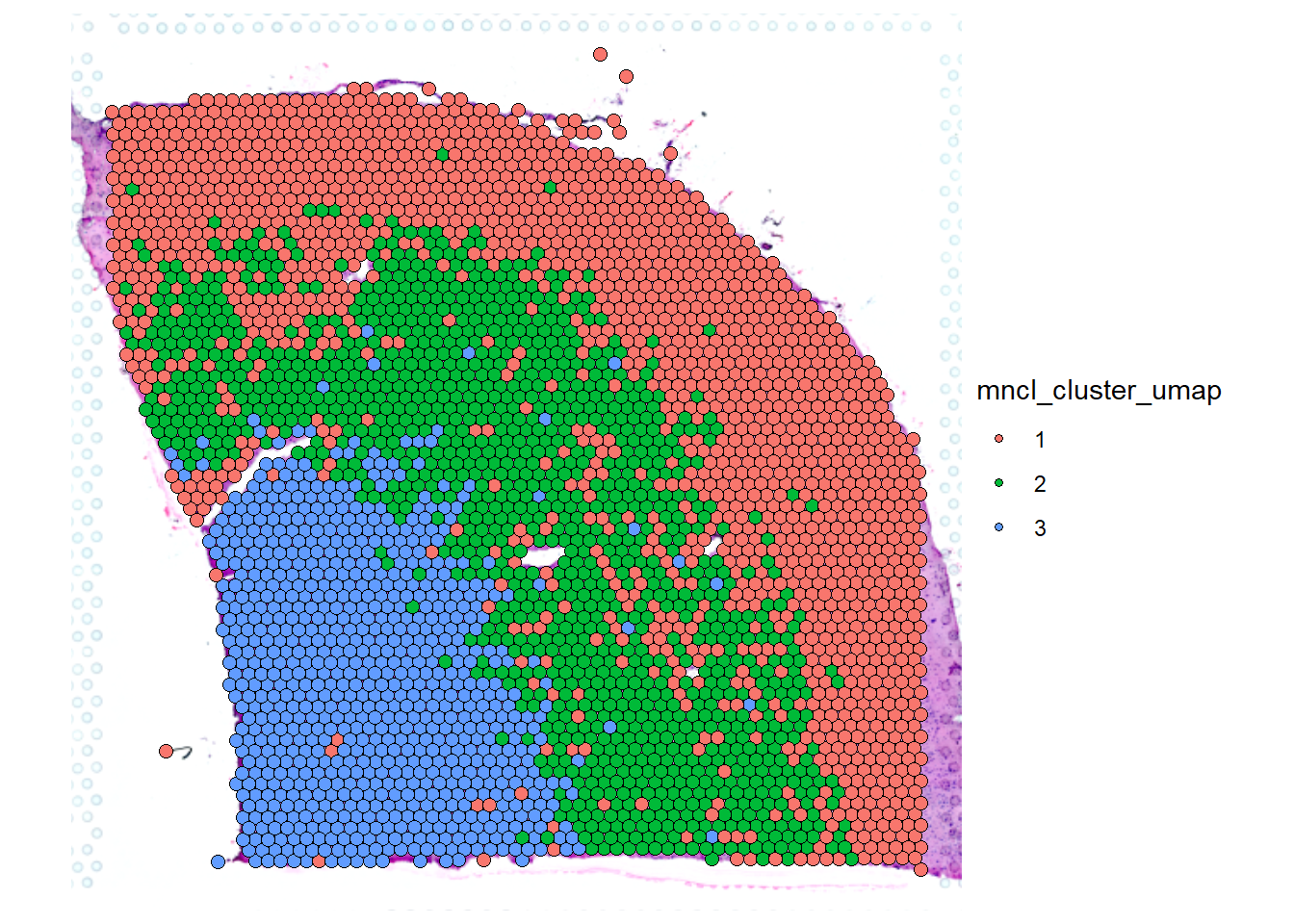
# applying the same pipeline to the clustering results
cluster_df <-
  clusters(cortex_cds, reduction_method = c("UMAP")) %>%
  as.data.frame() %>% # convert to data.frame
  magrittr::set_names("mncl_cluster_umap") %>% # provide feature name
  tibble::rownames_to_column("barcodes") # provide key variable

spata_obj <- addFeatures(object = spata_obj,
                         feature_names = "mncl_cluster_umap",
                         feature_df = cluster_df,
                         overwrite = T)

# visualize by surface-plotting
plotSurface(spata_obj, color_to = "mncl_cluster_umap", pt_size = 2.2, pt_clrp = "jama")
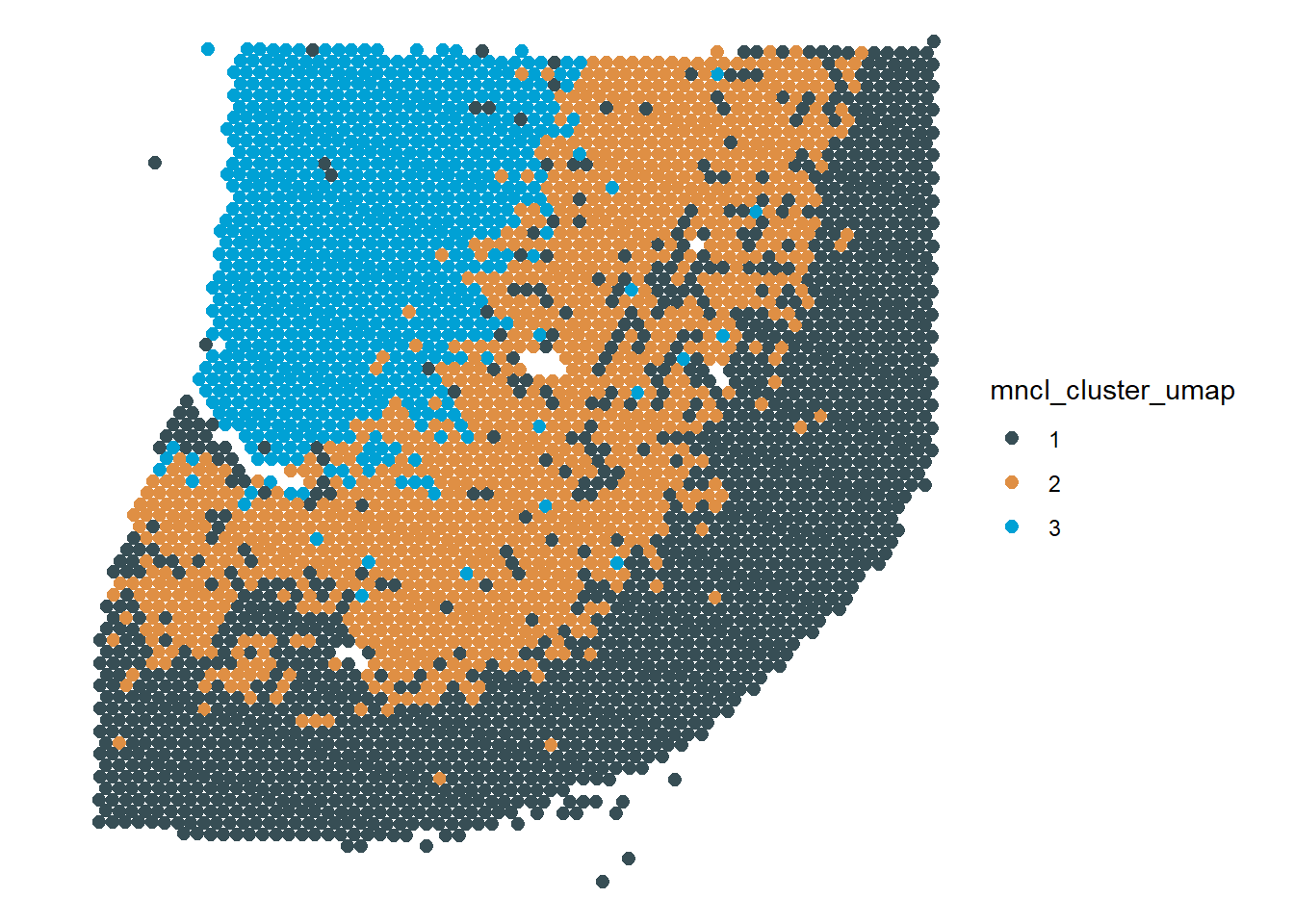
Figure 3 Add to and visualize monocle clustering with SPATA
Seurat
Seurat provides a variety of computational tools. Initiating a SPATA-object currently relies on most of it’s pre processing functions. If you want to switch from SPATA to Seurat make use of compileSeuratObject(). Similarly to initiateSpataObject() it is a wrapper around several preprocessing functions although it passes the feature-data of your spata-object to it in order not to loose your progress. It works in a similar fashion as compileCellDataSet().
cortex_seurat <- compileSeuratObject(object = spata_obj)
You can now continue your analysis with Seurat. Note that SPATA handles the image plotting differently which results in mirror-inverted plots.
# continue analysis adn plotting with seurat
Seurat::SpatialPlot(object = cortex_seurat, group.by = "mncl_cluster_umap")
Note that the meta.data slot of the seurat-object contains the barcodes- and the sample-variable of the spata-object it originally derived from.
# output
cortex_seurat@meta.data
As explained here all you need in order to make SPATA-extern obtained information available for SPATA-intern functions is a data.frame that contains either barcodes or coordinates as the key-variable. You can therefore pass your results from Seurat easily to SPATA in order to integrate those into your workflow.