Extract, join & add data
spata-extern-analysis.RmdThe framework in which SPATA operates invites you to extract data from the spata-object in order to do your own analysis apart from what SPATA currently offers. In order to do that you can make use of a variety of get- and joinWith-functions.
# load packages
library(SPATA)
library(magrittr)
library(ggplot2)
library(ggsci)

# load object
spata_obj <- loadSpataObject(input_path = "data/spata-obj-extern-analysis-tutorial.RDS")
Basic extracting functions
The following code introduces basic get-functions in order to obtain data from your spata-object.
The first two arguments are always:
-
objectThe spata-object of interest. -
of_sampleThe sample of interest. If not specified the first sample of all samples is chosen. If your spata-object contains only one sample you can therefore ignore this argument.
The code chunk below shows some examples.
# the essential data.frame
getSpataDf(spata_obj)
# dimensional reduction data
getUmapData(spata_obj)
# barcode spot coordinates
getCoordinates(spata_obj)
# feature data
getFeatureData(spata_obj)
Type SPATA::get in your console to skim SPATA’s namespace and to see all available get*()-functions.
The joinWith-family
As spatial transcriptomics analysis centers around the spatial expression of certain features it makes sense to start your spata-exclusive analysis by extracting the spatial coordinates of the sample of interest via getCoordinates().
# 1. get a data.frame that contains barcodes variables
spata_df <- getCoordinates(spata_obj, of_sample = "T275")

# output
spata_df
The coordinates themself aren’t particularly revealing which is why one needs to combine the coordinates of a barcode-spot with the respective information. As mentioned previously, SPATA is oriented towards the tidy-data approach which is demonstrated in particular by the joinWith()-family. It’s members leverage dplyr::left_join() to it’s fullest by making it ridiculously easy to extract your data in a barcode-spot related fashion. In order to get a detailed report about what every member of that family does run ?joinWith in your R-console. Although they might differ slightly in names and arguments they all follow the same concept. They
1.) take a data.frame containing the character-variables ‘barcodes’ and ‘sample’.
2.) extract the specified gene-, gene-set or feature information. (and perform normalization or smoothing if specified)
3.) return the data.frame with the specified variables included.
# 2. join this data.frame with additional information
joined_df <-
  joinWith(object = spata_obj,
           spata_df = spata_df,
           gene_sets = "HM_HYPOXIA", # expression values of the gene set Hallmark-Hypoxia
           features = "seurat_clusters", # cluster belonging according to package::Seurat
           verbose = FALSE)

# output
joined_df
It does not matter how many barcodes of a sample the particular data.frame contains. The specified variables are extracted and joined by their ‘barcodes’-variable whereby the barcodes inside the spata_df-data.frame are determining. The joinWith-family does not extend nor reduce the number of barcode-spots (or observations for that matter) but simply adds the desired information to the data.frame in form of additional variables using the barcodes as unique identifiers for every value.
As an example let us assume, that we have used createSegmentation()in order to partition our sample as depicted in the image below and we are only interested in analyzing the segment we called hypoxic-region due to it’s high expression levels for hypoxia-related genes.
plotSegmentation(spata_obj, of_sample = "T275")
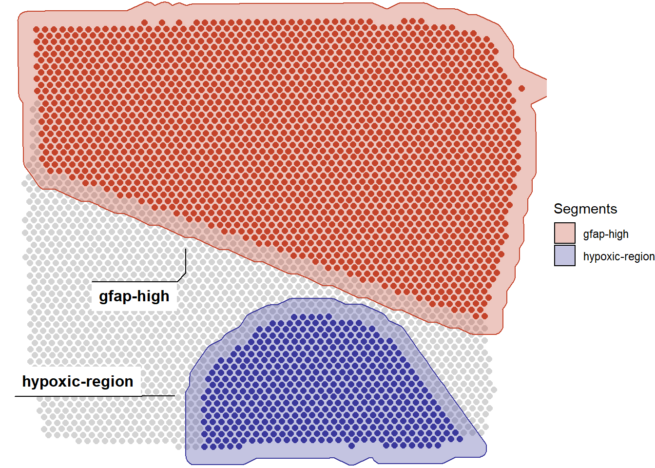
Figure 1. An example of segmentation
We therefore only extract the coordinates and barcodes that belong to the barcode-spots we included while drawing the hypoxic-region segment.
segm_coords <- getCoordinatesSegment(spata_obj, of_segment = "hypoxic-region", of_sample = "T275")

segm_joined <-
  joinWith(object = spata_obj,
           spata_df = segm_coords,
           gene_sets = "HM_HYPOXIA",
           genes = c("GFAP", "VEGFA"), # two genes
           features = "seurat_clusters", # all features
           verbose = FALSE)

# output
segm_joined
The number of variables of these data.frames can be expanded infinitely as long as there is a character-variable called ’barcodes’. Just specify it again as input for argument spata_df and tell joinWith() which information-variables it is supposed to add.
Add your results to SPATA
Let’s assume that our segm_joined-data.frame has undergone several analysis steps and you came up with a new clustering variable that you would like to integrate into the SPATA-workflow. The data.frame might now look somewhat like this:
It carries a new calculated feature that gives additional information about every barcode-spot. Whatever your analysis results in, as long as it is a variable in a data.frame that additionally contains barcodes of your spata-object in a ‘barcodes’-variable you can rejoin that variable to your spata-object to make it universally accessible for all SPATA-functions. Use addFeatures()for that matter.
# initial features in slot @fdata
getFeatureNames(spata_obj)
##           numeric           integer           numeric           numeric
##      "nCount_RNA"    "nFeature_RNA"      "percent.mt"      "percent.RB"
##            factor            factor         character
## "RNA_snn_res.0.8" "seurat_clusters"         "segment"
# add the feature spata_obj <- addFeatures(spata_obj, feature_names = "my_new_feature", feature_df = example_df) # new features in slot @fdata getFeatureNames(spata_obj)
##           numeric           integer           numeric           numeric
##      "nCount_RNA"    "nFeature_RNA"      "percent.mt"      "percent.RB"
##            factor            factor         character         character
## "RNA_snn_res.0.8" "seurat_clusters"         "segment"  "my_new_feature"
Note that the variable we just added carries information only for the barcode-spots that belong to the hypoxic-segment. For all other barcode-spots the newly added variable contains NAs.