Adding Data to SPATA2 objects • SPATA2

1. Introduction

While SPATA2 provides wrappers for multiple algorithms, you can always add data from external sources and packages. Depending on the kind of data you want to add, different functions are required.

library(SPATA2)
library(tidyverse)

# load SPATA2 inbuilt example data
object_t269 <- loadExampleObject("UKF269T")

2. Data matrices

Assuming you have a data matrix processed with functions from a different package (e.g. Seurat), you can add them to the SPATA2 object via the function addProcessedMatrix().

library(Seurat)

# create Seurat object from count matrix
count_mtr <- getCountMatrix(object_t269)

seurat_obj <- CreateSeuratObject(count_mtr)
seurat_obj <- NormalizeData(seurat_obj)
seurat_obj <- ScaleData(seurat_obj)

scaled_mtr <- GetAssayData(seurat_obj, layer = "scale.data")

# show a small subset of the scaled mtr 
scaled_mtr[1:5, 1:5]

##            AAACAAGTATCTCCCA-1 AAACACCAATAACTGC-1 AAACAGAGCGACTCCT-1
## AL669831.5        -0.13779796        -0.13779796        -0.13779796
## FAM87B            -0.03675644        -0.03675644        -0.03675644
## FAM41C            -0.11923196        -0.11923196        -0.11923196
## AL645608.1        -0.02790417        -0.02790417        -0.02790417
## KLHL17            -0.20169999         4.33113446        -0.20169999
##            AAACATTTCCCGGATT-1 AAACCCGAACGAAATC-1
## AL669831.5        -0.13779796        -0.13779796
## FAM87B            -0.03675644        -0.03675644
## FAM41C            -0.11923196        -0.11923196
## AL645608.1        -0.02790417        -0.02790417
## KLHL17            -0.20169999        -0.20169999

# add the processed matrix to SPATA2 object under the name 'scaled'
object_t269 <- 
  addProcessedMatrix(
    object = object_t269,
    proc_mtr = scaled_mtr,
    mtr_name = "scaled"  
    )

# the matrix is now accessible next to all other matrices
# ('counts' refers to the raw count matrix with which the SPATA2 object has been initated)
getMatrixNames(object_t269)

## [1] "counts" "scaled"

# check which matrix is currently active
activeMatrix(object_t269)

## [1] "counts"

# create a surface plot with EGFR expression using raw counts 
egfr_counts <- 
  plotSurface(object_t269, color_by = "EGFR") + 
  labs(subtitle = "Matrix: raw counts")

# activate the processes matrix to make functions pick it by default
object_t269 <- activateMatrix(object_t269, mtr_name = "scaled")
activeMatrix(object_t269)

## [1] "scaled"

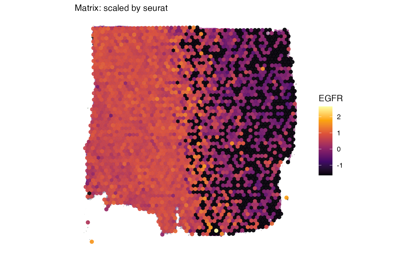
# create a surface plot with EGFR expression using scaled expression
egfr_scaled <- 
  plotSurface(object_t269, color_by = "EGFR") + 
  labs(subtitle = "Matrix: scaled by seurat")

# show plots
egfr_counts
egfr_scaled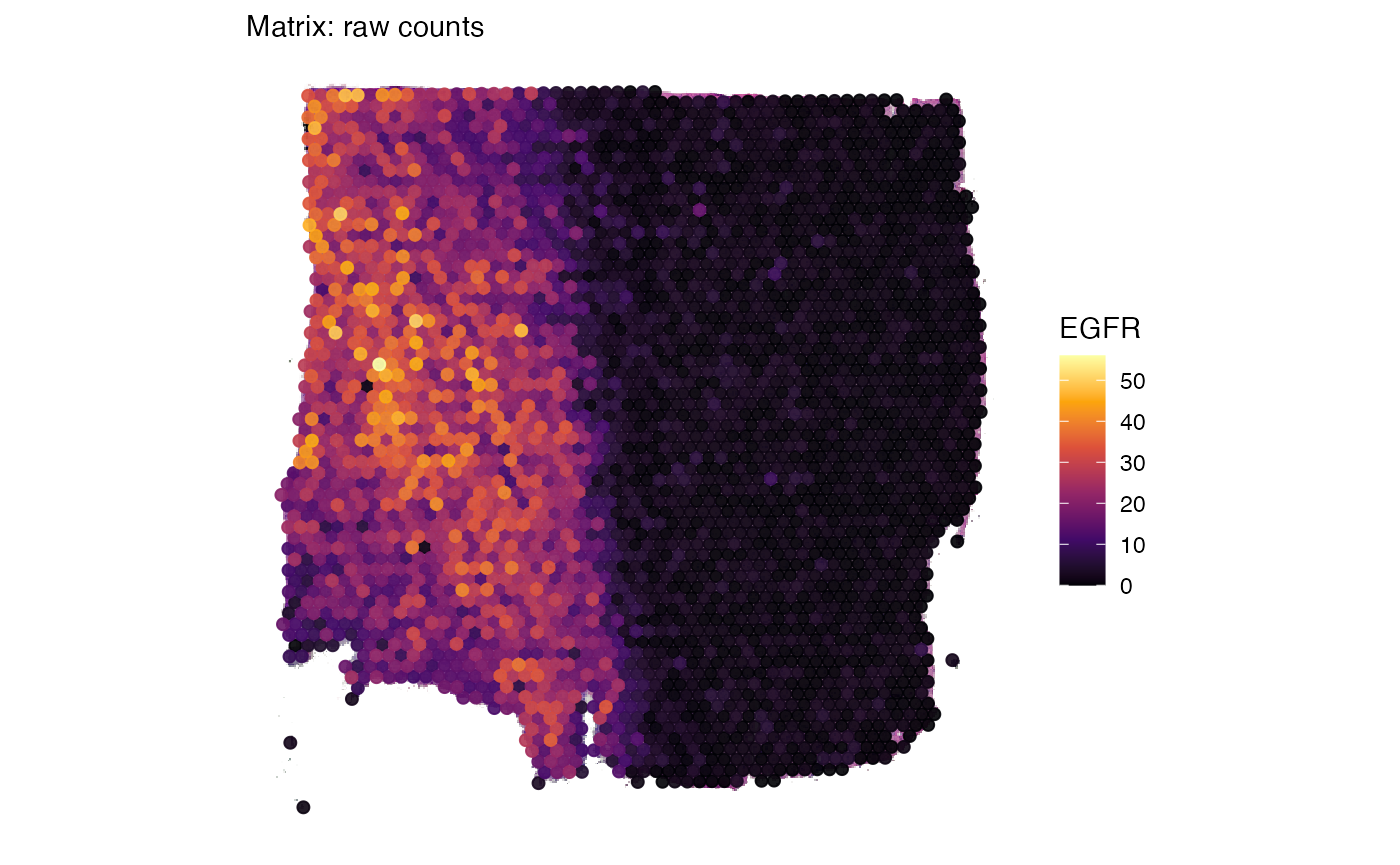

3. Meta features

Features that are not raw or processed molecular counts, like clustering or certain scores, are stored in the meta data.frame of the SPATA2 object, as obtained by getMetaDf(). SPATA2 intern functions like runBayesSpaceClustering() or runCNV() add the results automatically to this data.frame. The following code chunk creates a data.frame of meta SPATA2 extern created meta features that can be added to the SPATA2 object.

seurat_obj <- FindVariableFeatures(seurat_obj)
seurat_obj <- RunPCA(seurat_obj)
seurat_obj <- FindNeighbors(seurat_obj)
seurat_obj <- FindClusters(seurat_obj)

## Modularity Optimizer version 1.3.0 by Ludo Waltman and Nees Jan van Eck
## 
## Number of nodes: 3217
## Number of edges: 108933
## 
## Running Louvain algorithm...
## Maximum modularity in 10 random starts: 0.8293
## Number of communities: 11
## Elapsed time: 0 seconds

# add rownames as 'barcodes' variable 
seurat_meta_df <- 
  tibble::rownames_to_column(seurat_obj@meta.data, var = "barcodes") %>% 
  tibble::as_tibble()

# show meta df
seurat_meta_df

## # A tibble: 3,217 × 6
##    barcodes   orig.ident nCount_RNA nFeature_RNA RNA_snn_res.0.8 seurat_clusters
##    <chr>      <fct>           <dbl>        <int> <fct>           <fct>          
##  1 AAACAAGTA… SeuratPro…       1614          842 0               0              
##  2 AAACACCAA… SeuratPro…      10498         3211 10              10             
##  3 AAACAGAGC… SeuratPro…       1258          739 1               1              
##  4 AAACATTTC… SeuratPro…       2387         1226 0               0              
##  5 AAACCCGAA… SeuratPro…       3070         1373 0               0              
##  6 AAACCGGGT… SeuratPro…      14562         3579 5               5              
##  7 AAACCGTTC… SeuratPro…       8014         2610 3               3              
##  8 AAACCTAAG… SeuratPro…       4476         1945 9               9              
##  9 AAACCTCAT… SeuratPro…       9823         2818 5               5              
## 10 AAACGAGAC… SeuratPro…        584          415 1               1              
## # ℹ 3,207 more rows

The meta data.frame from the Seurat object contains cluster results as well as summarizing numeric variables like nCount_RNA and nFeature_RNA. These variables can be added to the SPATA2 object and are afterwards accessible with all SPATA2 functions.

# add features from the data.frame 
object_t269 <- 
  addFeatures(
    object = object_t269,
    feature_df = seurat_meta_df, 
    feature_names = c("nCount_RNA", "seurat_clusters"), 
    overwrite = TRUE
    )

# once added, they are accessible for all SPATA2 functions 
plotSurface(object_t269, color_by = "nCount_RNA")  
plotSurface(object_t269, color_by = "seurat_clusters", pt_clrp = "sifre")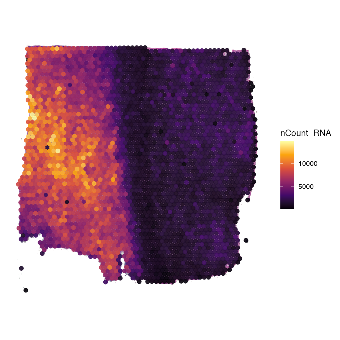

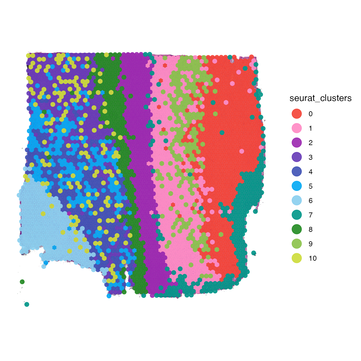
Grouping variables such as the seurat_clusters variable can be used for comparative analysis.

plotBoxplot(object_t269, variables = "nCount_RNA", across = "seurat_clusters", clrp = "sifre") + 
 legendNone() + 
 labs(x = "seurat clusters")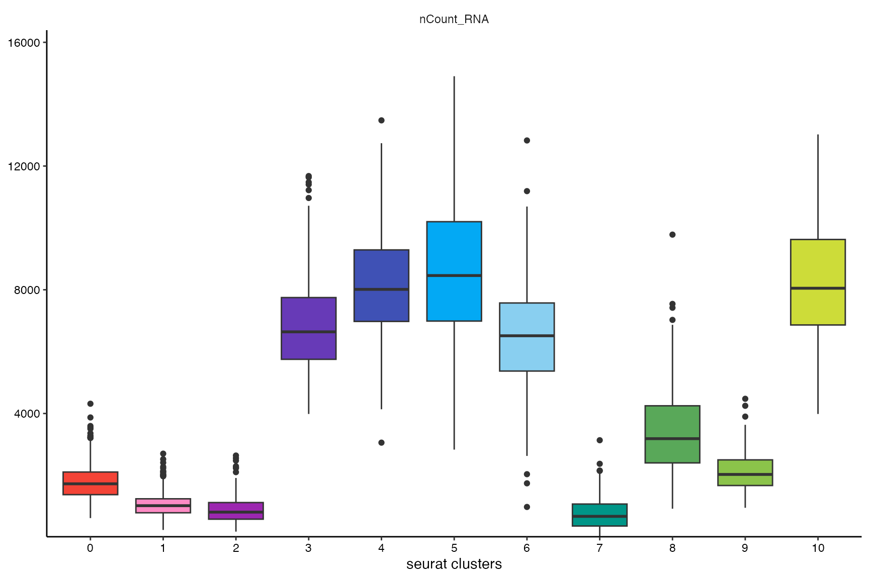

4. Images

To learn how to register additional images in the SPATA2 object please refer to the vignette about image handling in SPATA2.