Clustering

1. Introduction

Grouping variables divide the observations of the sample into groups whose properties can be compared against each other. For instance, the grouping of observations can be the result of clustering algorithms or manual spatial segmentation. This tutorial shows how to apply and add clustering in SPATA2.

# load required packages
library(SPATA2)
library(SPATAData)
library(tidyverse)

# load SPATA2 object
object_t313 <- downloadSpataObject(sample_name = "UKF313T")

# alternatively, use diet version (results might differ slightly)
object_t313 <- loadExampleObject(sample_name = "UKF313T", process = TRUE)

# show sample
plotImage(object_t313)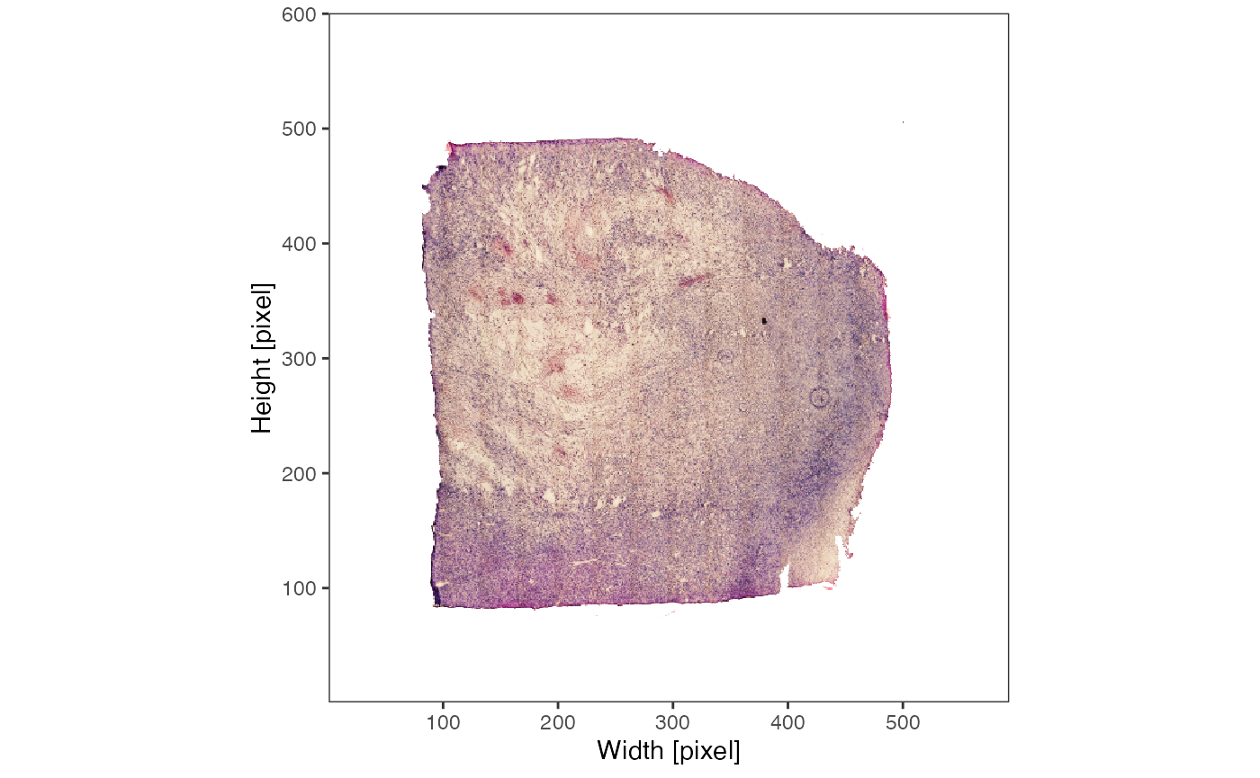

2. Clustering within SPATA2

There are several algorithms out there that can be used to divide your sample into subgroups. SPATA2 provides wrappers around several clustering algorithms. Cluster algorithms that add their results immediately to the SPATA2 object are prefixed with with run-* and suffixed with *-Clustering(). E.g. runBayesSpaceClustering(), runKmeansClustering(), runSeuratClustering().

# current grouping options 
getGroupingOptions(object_t313)

##           factor 
## "tissue_section"

Argument name or naming specifies the name of the output grouping variable. The resulting grouping variable names are available with getGroupingOptions().

# run the pipeline
object_t313 <- 
  runBayesSpaceClustering(
    object = object_t313, 
    name = "bayes_space", # the name of the output grouping variable
    qs = 5
  )

# run PCA based on which clustering is conducted
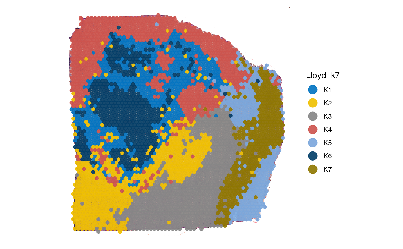
object_t313 <- runPCA(object_t313, n_pcs = 20)

object_t313 <- 
  runKmeansClustering(
    object = object_t313, 
    ks = c(7, 8), 
    methods_kmeans = "Lloyd"
  )

# results are immediately stored in the objects feature data
getGroupingOptions(object_t313)

##            factor            factor            factor            factor 
##  "tissue_section" "seurat_clusters"     "bayes_space"        "Lloyd_k7" 
##            factor 
##        "Lloyd_k8"

# left plot
plotSurface(
  object = object_t313, 
  color_by = "bayes_space", 
  pt_clrp = "uc"
)

# right plot
plotSurface(
  object = object_t313, 
  color_by = "Lloyd_k7",
  pt_clrp = "jco"
  )

3. Clustering outside of SPATA2

Clustering can result from a multitude of cluster algorithms. If they are not implemented in SPATA2 functions you can add them using the addFeatures() function.

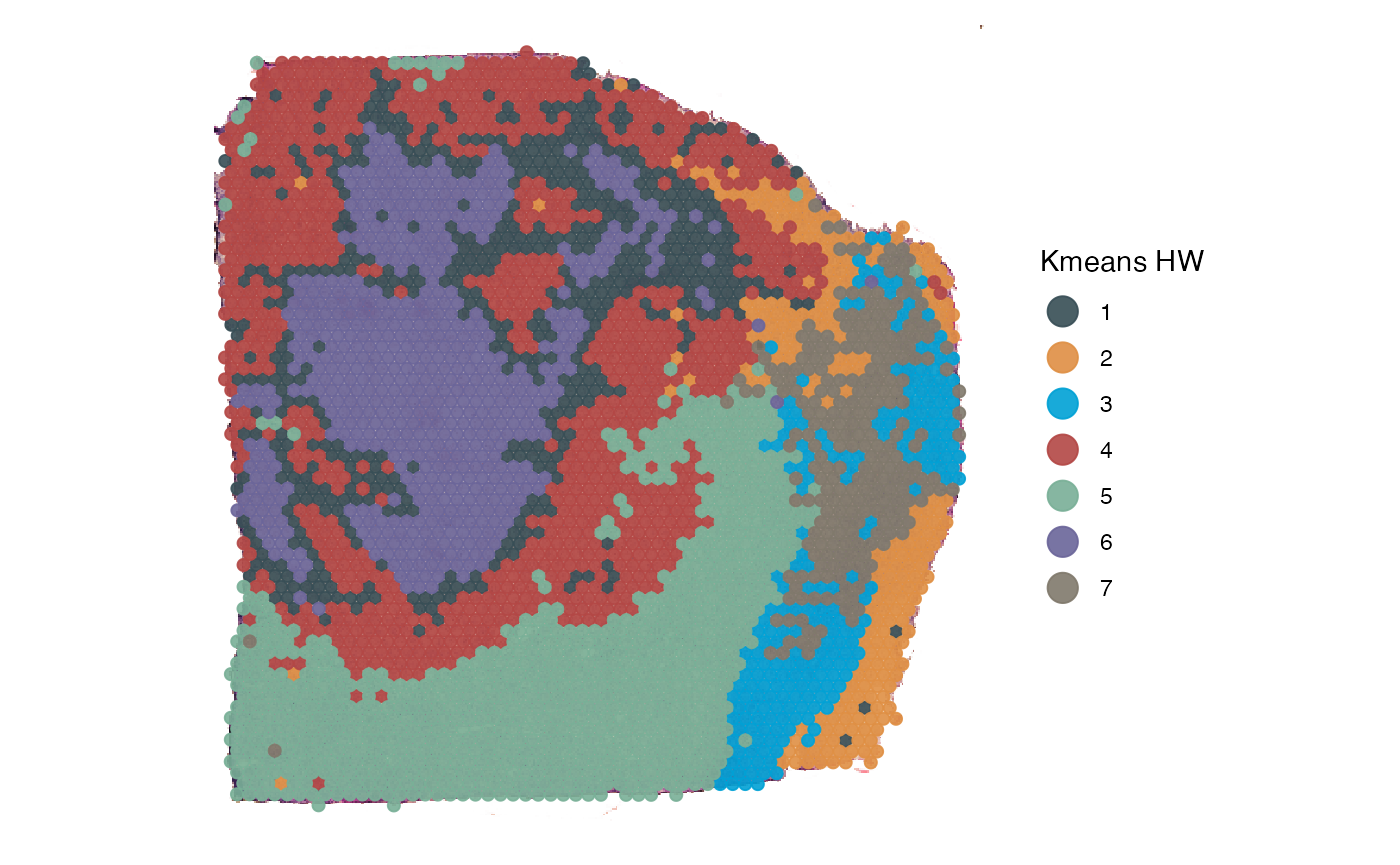
# uses kmeans outside of SPATA2
kmeans_res <- 
  stats::kmeans(
    x = getPcaMtr(object_t313), 
    centers = 7, 
    algorithm = "Hartigan-Wong"
  )

head(kmeans_res[["cluster"]])

## AAACAAGTATCTCCCA-1 AAACAATCTACTAGCA-1 AAACACCAATAACTGC-1 AAACAGAGCGACTCCT-1 
##                  3                  5                  6                  3 
## AAACAGCTTTCAGAAG-1 AAACAGGGTCTATATT-1 
##                  1                  6

cluster_df <- 
  as.data.frame(kmeans_res[["cluster"]]) %>% 
  tibble::rownames_to_column(var = "barcodes") %>% 
  magrittr::set_colnames(value = c("barcodes", "kmeans_4_HW")) %>% 
  tibble::as_tibble()

cluster_df[["kmeans_4_HW"]] <- as.factor(cluster_df[["kmeans_4_HW"]])

cluster_df

## # A tibble: 3,517 × 2
##    barcodes           kmeans_4_HW
##    <chr>              <fct>      
##  1 AAACAAGTATCTCCCA-1 3          
##  2 AAACAATCTACTAGCA-1 5          
##  3 AAACACCAATAACTGC-1 6          
##  4 AAACAGAGCGACTCCT-1 3          
##  5 AAACAGCTTTCAGAAG-1 1          
##  6 AAACAGGGTCTATATT-1 6          
##  7 AAACATGGTGAGAGGA-1 4          
##  8 AAACCCGAACGAAATC-1 2          
##  9 AAACCGGGTAGGTACC-1 6          
## 10 AAACCGTTCGTCCAGG-1 1          
## # ℹ 3,507 more rows

Only requirement is a barcodes variable to map the groups to the observations. Note that a variable must be of class factor in order to be recognized as a grouping variable.

# grouping options before adding
getGroupingOptions(object_t313)

##            factor            factor            factor            factor 
##  "tissue_section" "seurat_clusters"     "bayes_space"        "Lloyd_k7" 
##            factor 
##        "Lloyd_k8"

# add the cluster results to the meta features
object_t313 <- 
  addFeatures(
    object = object_t313,
    feature_df = cluster_df
    )

# grouping options names afterwards
getGroupingOptions(object_t313)

##            factor            factor            factor            factor 
##  "tissue_section" "seurat_clusters"     "bayes_space"        "Lloyd_k7" 
##            factor            factor 
##        "Lloyd_k8"     "kmeans_4_HW"

Continue by visualizing your results or by investigating their transcriptional characteristics using differential expresseion analysis (DEA)).

plotSurface(
  object = object_t313,
  color_by = "kmeans_4_HW",
  pt_clrp = "jama"
  ) +
  labs(color = "Kmeans HW")