Differential Expression Analysis (DEA) • SPATA2

1. Introduction

Differential expression analysis (DEA) aims to discover quantitative changes in gene expression levels between defined experimental groups. Grouping information is stored in form of grouping variables in the meta data of SPATA2 object. This includes all SPATA2 intern generated grouping options such as spatial segmentation and clustering as well as any other grouping variable that has been added via addFeatures().

# load required packages
library(SPATA2)
library(tidyverse)

# load SPATA2 inbuilt example data
object_t269 <- loadExampleObject("UKF269T", process = TRUE, meta = TRUE)

# plot histology 
plotSurface(object_t269, color_by = "histology", pt_clrp = "npg")

# plot bayes space cluster
plotSurface(object_t269, color_by = "bayes_space", pt_clrp = "uc")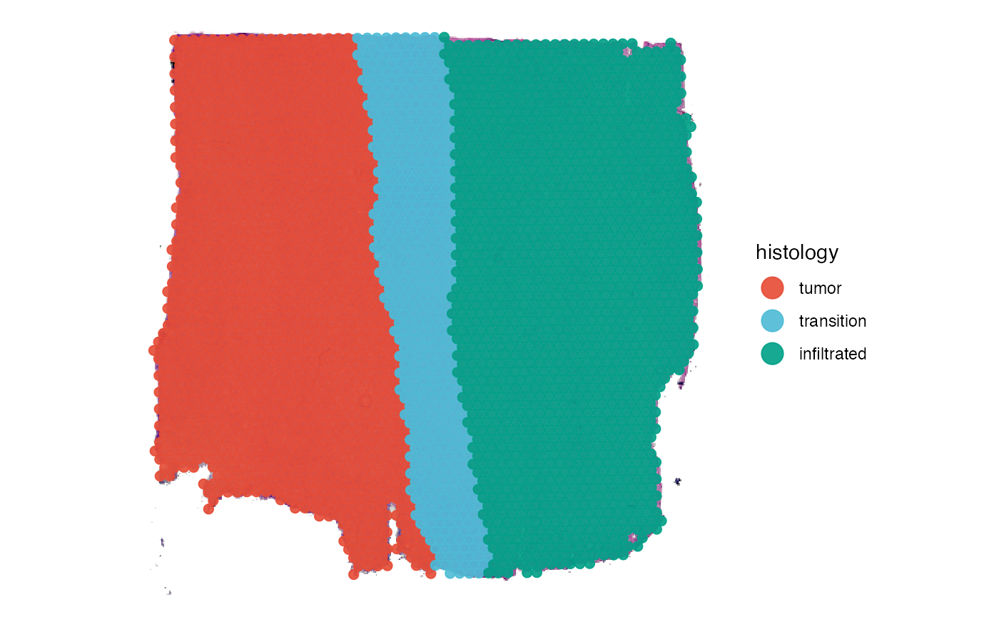

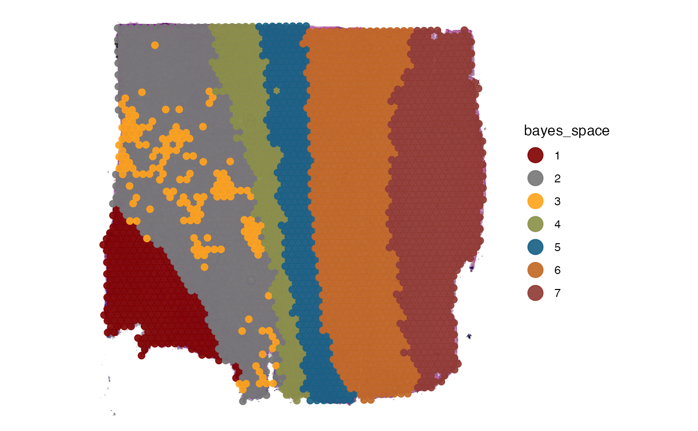
The function getGroupingOptions() returns the variable names based on which DEA can be conducted. This vignette conducts differential expression analysis based on the histological grouping. You can exchange ‘histology’ with ‘bayes_space’ whenever the grouping is specified to use the clustering results.

getGroupingOptions(object_t269)

##            factor            factor            factor            factor 
##  "tissue_section" "seurat_clusters"       "histology"     "bayes_space"

2. Running the analysis

SPATA2 uses the function Seurat::FindAllMarkers() for differential expression analysis. It’s output is a data.frame in which each row corresponds to a gene that turned out to be a marker gene for one of the identity groups. Additional variables provide information about it’s p-value, adjusted p-value, logFold change etc. runDEA() does not alter the output but stores it in the SPATA2 object.

object_t269 <- runDEA(object = object_t269, across = "histology", method = "wilcox")

3. Extracting results

There are two main functions with which you can manually extract the DEA results desired. First, getDeaResultsDf() returns the original resulting data.frame of Seurat::FindAllMarkers(). getDeaGenes() returns a vector of gene names.

# extract the complete data.frame
dea_df <- 
  getDeaResultsDf(
    object = object_t269, 
    across = "histology"
  )

nrow(dea_df)

## [1] 22298

head(dea_df)

## # A tibble: 6 × 7
##      p_val avg_log2FC pct.1 pct.2 p_val_adj histology gene     
##      <dbl>      <dbl> <dbl> <dbl>     <dbl> <fct>     <chr>    
## 1 3.26e-17       7.54 0.037     0  4.89e-13 tumor     SAA2     
## 2 7.28e-23       7.07 0.05      0  1.09e-18 tumor     NODAL    
## 3 1.55e-19       6.85 0.042     0  2.33e-15 tumor     MPZL2    
## 4 7.17e-19       6.69 0.041     0  1.08e-14 tumor     LINC02308
## 5 7.09e-18       6.61 0.038     0  1.06e-13 tumor     CD48     
## 6 3.26e-17       6.56 0.037     0  4.89e-13 tumor     HOXA-AS2

Using the arguments across_subset, min_lfc, n_highest_lfc, max_adj_pval, n_lowest_pval the output of the function can be adjusted to specific questions.

# e.g. top 10 genes for histology area 'tumor' 
getDeaResultsDf(
  object = object_t269, 
  across = "histology",
  across_subset = "transition", # the group name(s) of interest,
  n_highest_lfc = 10, # top ten genes
  max_adj_pval = 0.01 # pval must be lower or equal than 0.01
)

## # A tibble: 10 × 7
##        p_val avg_log2FC pct.1 pct.2 p_val_adj histology  gene     
##        <dbl>      <dbl> <dbl> <dbl>     <dbl> <fct>      <chr>    
##  1 8.53e-  8       7.98 0.01  0     1.28e-  3 transition CPEB1-AS1
##  2 1.21e- 11       4.59 0.042 0.006 1.82e-  7 transition SGK2     
##  3 8.16e- 30       4.40 0.111 0.016 1.22e- 25 transition GPIHBP1  
##  4 2.18e- 20       4.34 0.075 0.011 3.28e- 16 transition FAM95C   
##  5 1.00e- 10       4.07 0.04  0.006 1.50e-  6 transition HOXD1    
##  6 6.57e- 72       4.03 0.303 0.057 9.86e- 68 transition GJB1     
##  7 6.05e- 12       3.90 0.054 0.011 9.08e-  8 transition SMIM6    
##  8 1.65e-  8       3.70 0.061 0.018 2.48e-  4 transition PIEZO2   
##  9 4.50e- 15       3.69 0.088 0.022 6.75e- 11 transition LRP2     
## 10 2.39e-168       3.68 0.72  0.2   3.58e-164 transition MAG

4. Visualize results

4.1 Heatmaps

plotDeaHeatmap() visualizes the results of DEA by using to the results you would extract with getDeaResultsDf().

hm <- 
  plotDeaHeatmap(
    object = object_t269, 
    across = "histology",
    clrp = "npg",
    n_highest_lfc = 10, # subset genes
    n_bcs = 100
  )

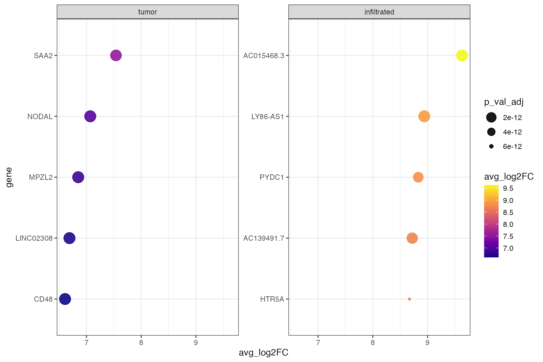
hm

4.2 Dotplots

plotDeaDotPlot() visualizes the results of DEA either by group…

plotDeaDotPlot(
  object = object_t269, 
  across = "histology",
  across_subset = c("tumor", "infiltrated"), # specify single groups if desired
  n_highest_lfc = 5,
  by_group = TRUE, 
  scales = "free_y", 
  nrow = 1
)

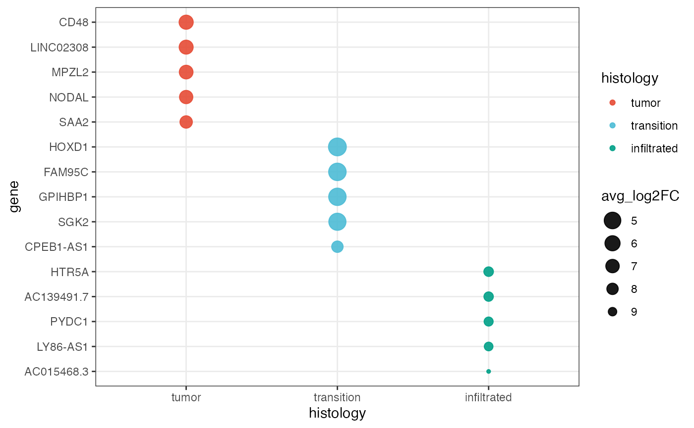
… or with all groups together.

plotDeaDotPlot(
  object = object_t269, 
  across = "histology",
  color_by = "histology",
  pt_clrp = "npg",
  size_by = "avg_log2FC",
  n_highest_lfc = 5, 
  by_group = FALSE
)

4.3 Box- and Violinplots

There are additional ways to visualize the results of your DEA. As with almost all plotting functions in SPATA2 a vector of gene names is necessary for the function to know which genes to plot. getDeaGenes() is the second function to extract DEA results and a wrapper around getDeaResultsDf() that returns a vector gene names.

genes_of_interest <-
  getDeaGenes(
    object = object_t269,
    across = "histology", # the grouping variable
    method_de = "wilcox", # the method with which the results were computed
    n_highest_lfc = 10, 
    max_adj_pval = 0.001
  )

head(genes_of_interest) # first six

##       tumor       tumor       tumor       tumor       tumor       tumor 
##      "SAA2"     "NODAL"     "MPZL2" "LINC02308"      "CD48"  "HOXA-AS2"

tail(genes_of_interest) # last six

## infiltrated infiltrated infiltrated infiltrated infiltrated infiltrated 
##     "HTR5A"     "CRHR2"    "CACNG2"    "TRIM54"     "ACTC1"    "KRT222"

A vector of gene names as returned by getDeaGenes() is a perfectly valid input for other plotting functions.

top_5_markers_269 <- 
  getDeaGenes(
    object = object_t269,
    across = "histology",
    n_lowest_pval = 5, 
    min_lfc = 0.1 # set min_lfc! else downregulated genes are included
    ) 

top_5_markers_269

##       tumor       tumor       tumor       tumor       tumor  transition 
##    "IGFBP2" "LINC01445"     "SOCS2"       "TNC"     "MATN2"       "MAG" 
##  transition  transition  transition  transition infiltrated infiltrated 
##      "MOBP"        "TF"      "PLP1"       "MBP"       "CCK"     "VSNL1" 
## infiltrated infiltrated infiltrated 
##      "NRGN"     "OLFM1"   "SLC17A7"

# plot results for t269
plotBoxplot(
  object = object_t269,
  variables = top_5_markers_269,
  across = "histology", 
  clrp = "npg",
  nrow = 3 
  ) + 
  theme(axis.text.x = element_blank(), axis.ticks.x = element_blank()) +
  legendTop()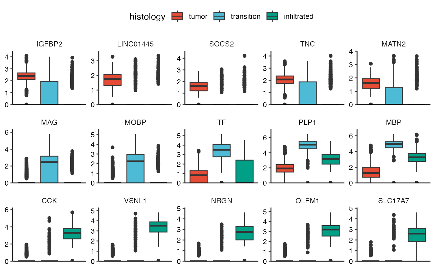

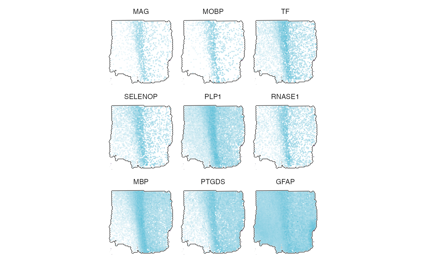
4.4 Surface plots

getDeaGenes() complements plotSurfaceComparison().

# top 9 markers for transition area
transition_markers <- 
  getDeaGenes(object_t269, across = "histology", across_subset = "transition", n_lowest_pval = 9)

plotSurfaceComparison(
  object = object_t269, 
  color_by = transition_markers,
  pt_clrsp = color_vector("npg")[2], # plot cluster color against white
  outline = TRUE,
  nrow = 3
  ) + 
  legendNone()