Initiation & Preprocessing: VisiumHD • SPATA2

1. Initiation

To initiate a SPATA2 object directly from the Visium output use the function initiateSpataObjectVisiumHD(). This example vignette uses data from an example data set provided by 10X Genomics. You can download the folder here.

Note: It is crucial to install the package arrow in a way that arrow::read_parquet() works. There are several ways. Installing the package with install.packages('arrow', repos = 'https://apache.r-universe.dev') worked reliably for us.

library(SPATA2)
library(tidyverse)

object <- 
  initiateSpataObjectVisiumHD(
    sample_name = "HumanPancreasHD", 
    directory_visium = "my/path/to/VisiumHD_folder" # adjust to your liking 
  )

# show overview
object

## An object of class SPATA2
## Sample: HumanPancreasHD 
## Size: 106574 x 18085 (spots x molecules)
## Memory: 663.77 Mb
## Platform: VisiumHD (Resolution: 16um) 
## Molecular assays (1):
## 1. Assay
##  Molecular modality: gene
##  Distinct molecules: 18085
##  Matrices (1):
##  -counts (active)
## Registered images (2):
## - hires (6000x5968 px, not loaded)
## - lowres (600x597 px, active, loaded)
## Meta variables (2): sample, tissue_section

While VisiumHD offers standard resolutions with 16um, 8um and 2um, the squared nature of the grid of spots allows to analyze data in individual resolutions. Hence, if you want to analyze your data in resolution 10um, 24um, 30um or 40um (etc.) you can specify that and the function reduceResolutionVisiumHD() works in the background of initiateSpataObjectVisiumHD() to create the resolution of your liking. Read more on that in this vignette.

Furthermore, you can adjust the resolutions with which images are used. Particularly, the hires image of the VisiumHD platform is often too large for R to handle smoothly since R is not particularly efficient when it comes to handling images of a certain size. This resizing functionality allows you to adjust the size in which the image is handled when used in order to optimize the ratio between image resolution and computational performance. The function required is resizeImage() which can be called after initiation or used during initiation with the resize_images argument.

# example genes 
example_genes <- 
  c(
    'INS', 'REG3A', 'TTR', 'GCG', 'GHRL', 'SST', 'VIP', 'PPY', 'CARTPT', 'REG1B', 
    'NPY', 'REG3G', 'ALDOB', 'PCSK1N', 'IAPP', 'IGKC', 'DKK4', 'CHGA', 'IGHA1', 
    'CPA3', 'PLA2G2A', 'GAL', 'RBP4', 'SLC30A8', 'HBA2'
    )

# example object using the resize options
object_resized <- 
  initiateSpataObjectVisiumHD(
    sample_name = "HumanPancreasHD", 
    directory_visium = "my/path/to/VisiumHD_folder", 
    square_res = "20um",
    genes = example_genes, 
    unload = FALSE, 
    resize_images = list(hires = 0.5, lowres = 0.5)
  )

# show object
object_resized

## An object of class SPATA2
## Sample: HumanPancreasHD 
## Size: 68558 x 25 (spots x molecules)
## Memory: 1.31 Gb
## Platform: VisiumHD (Resolution: 20um) 
## Molecular assays (1):
## 1. Assay
##  Molecular modality: gene
##  Distinct molecules: 25
##  Matrices (1):
##  -counts (active)
## Registered images (2):
## - hires (3000x2984 px, loaded)
## - lowres (300x298.5 px, active, loaded)
## Meta variables (5): sample, square_exp, square_count, square_perc, tissue_section

Notice the different image resolutions between object and object_resized in the printed object summary. Images can be plotted with plotImage().

# left plot
plotImage(object_resized, img_name = "lowres")

# right plot
plotImage(object_resized, img_name = "hires")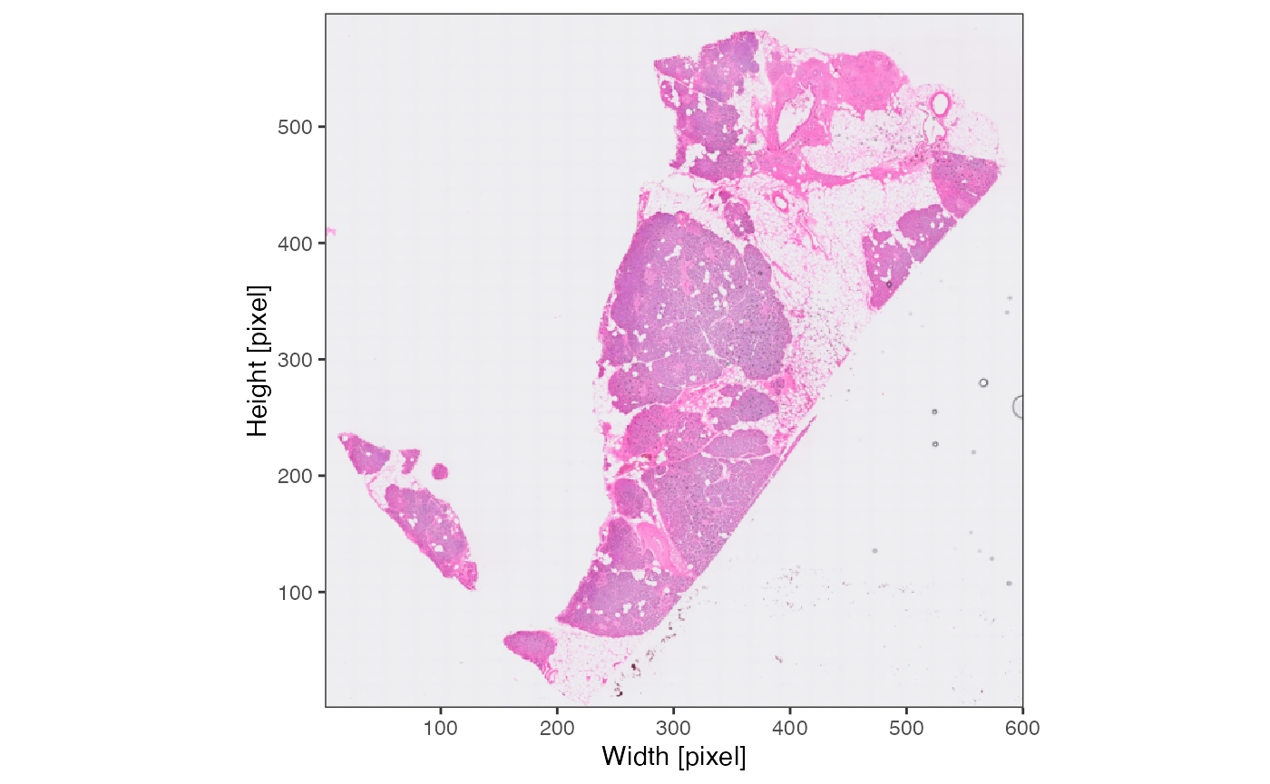

For this vignette, we’ll use the 16um object, simply stored in object.

2. Image processing

Image processing is not required. However, it facilitates the integration of histological features as displayed by the histology image, the Visium platform allows to integrate. The goal of image processing is to identify the precise spatial outline of the tissue on the histology slide. The function processImage() is a wrapper around identifyPixelContent() and identifyTissueOutline(..., method = "image"). Please refer to the documentation of either function to obtain more information.

# by default, the active image is always used
# you might need to adjust sigma, frgmt_threshold and other parameters to optimize results 
object <- identifyPixelContent(object, frgmt_threshold = c(0.01,0.05))

object <- identifyTissueOutline(object, method = "image")

The results of identifyPixelContent() can be plotted with plotImageMask() and plotPixelContent().

plotImageMask(object)

plotPixelContent(object, clrp = "jco")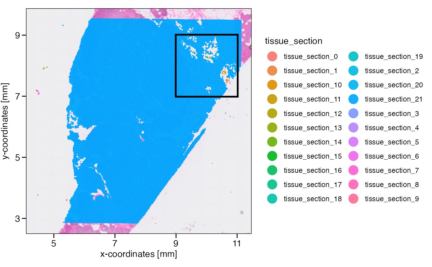

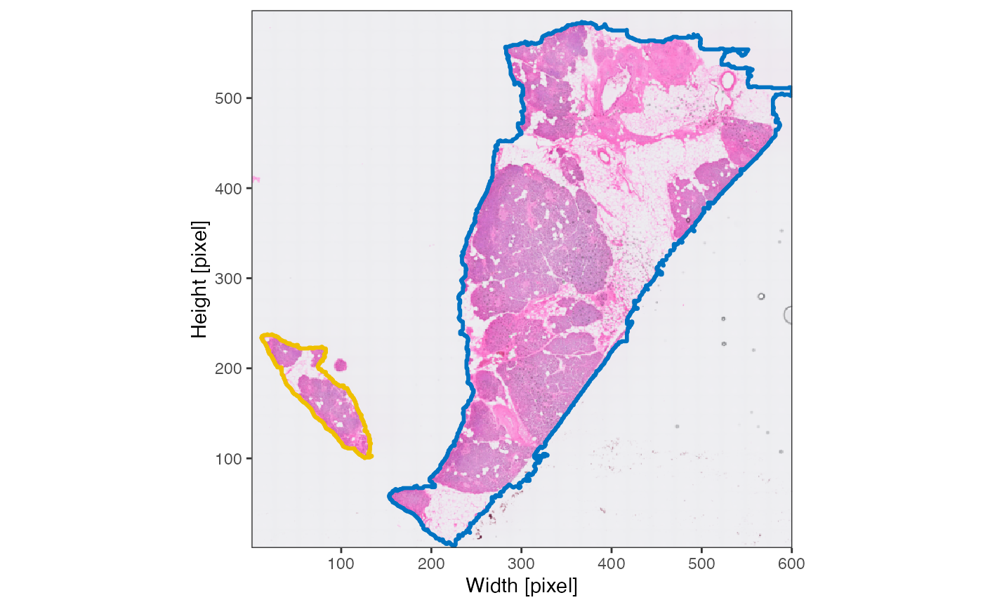
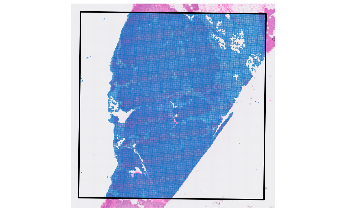
The results of identifyTissueOutline(..., method = "image") are best visualized by setting outline = TRUE with the plotImage() function.

# get colors of one of the known color palettes
cvec <- color_vector("jco")

# left plot
plotImage(object)

# right plot
plotImage(object, outline = TRUE, line_size = 1, line_color = cvec[1], fragments = cvec[2])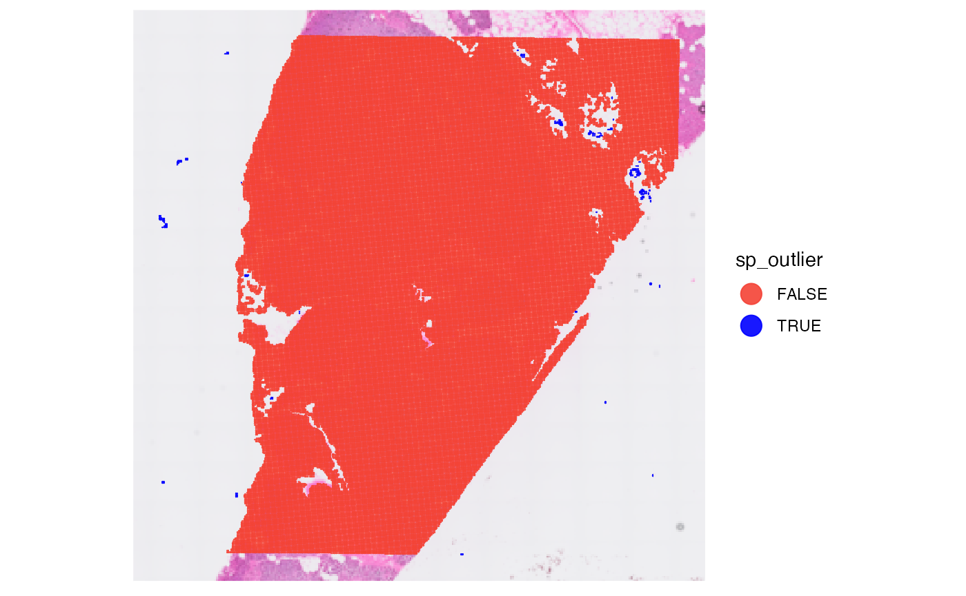

Note, that the tissue fragment identified on the left of the image is located within the capture area of the Visium slide. Hence, it won’t be of importance when it comes to analyzing gene expression.

# left plot
plotImage(object, outline = TRUE, line_size = 1, line_color = cvec[1], fragments = cvec[2]) + 
  ggpLayerPoints(object, pt_clr = cvec[1], pt_alpha = 0.5, use_scattermore = T) + 
  ggpLayerFrameByImage(object) + 
  ggpLayerCaptureArea(object) 

# right plot
plotSurface(object, pt_clr = cvec[1], pt_alpha = 0.5) + 
  ggpLayerCaptureArea(object)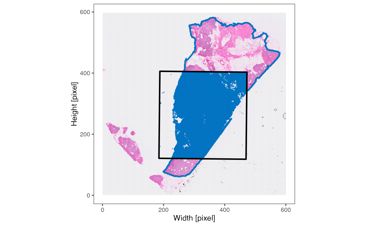

3. Spatial processing

This step should not be skipped! Many functions in SPATA2 need to know where the edge of the tissue section is and they need to know if there are multiple tissue sections. This kind of data is not provided with the standard output of most platforms and needs to be computed. With spatial processing we particularly refer to the identification of the tissue edge and spatial outliers - observations that are part of the data set but lie too far away from the contiguous tissue section to be considered part of the data set that is of actual interest. In case of the VisiumHD platform they are usually artefacts. The function identifyTissueOutline(..., method = "obs") uses the DBSCAN algorithm to identify potential spatial outliers. The tutorial for non-HD Visium exemplifies that.

# this is the default input for the visium platform and has already been 
# called in initiateSpataObjectVisiumHD(). 
# if the results do not satisfy you, you can run it over and over again with 
# different parameter inputs 
object <- identifyTissueOutline(object, method = "obs", eps = "20um", minPts = 3)

xrange <- c("9mm", "11mm")
yrange <- c("7mm", "9mm")

axes_layer <- ggpLayerAxesSI(object, breaks = str_c(c(3, 5, 7, 9, 11), "mm"))
rect_layer <- ggpLayerRect(object, xrange = xrange, yrange = yrange)

# left plot
plotSurface(object, color_by = "tissue_section") + 
  axes_layer +
  rect_layer

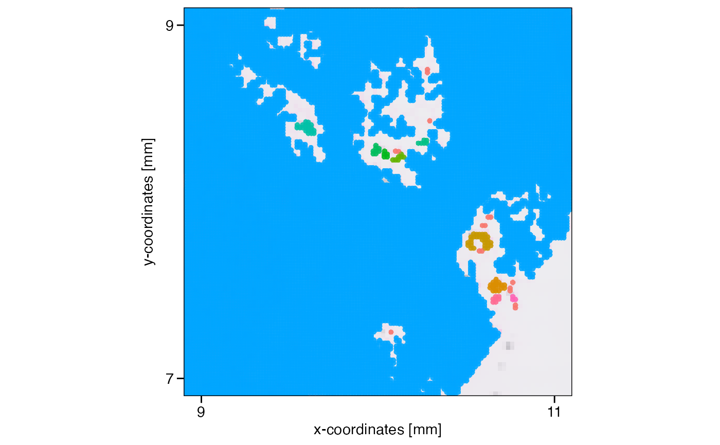
# right plot (zoomed in on rectangular)
plotSurface(object, color_by = "tissue_section", xrange = xrange, yrange = yrange) + 
  axes_layer + 
  legendNone()

What has been defined as tissue_section_0 could not be assigned to a tissue section and is always considered a spatial outlier. Furthermore, observations of tissue sections that are too small are labeled as spatial outliers, too. What defines too small can be set with min_section which takes a numeric value defining the minimal number of observations in order for a tissue section to be considered large enough. Note that you can also use the results of identifyTissueOutline(..., method = 'image') for spatial outlier detection and removal or combine the results of both methods by setting method = 'image' or method = c('image', 'obs'). You can play around with these parameters using identifySpatialOutliers() over and over again since the resulting sp_outlier meta variable is simply overwritten. Manual adjustment of this variable is always possible using getMetaDf() and addFeatures(..., overwrite = TRUE).


# min_section = 1% of all observations
min_section <- nObs(object)*0.01

min_section
## [1] 1065.74

# uses the results of identifyTissueOutline() to create a logical variable called sp_outlier
object <- identifySpatialOutliers(object, method = "obs", min_section = min_section)

plot_with_outliers <- plotSurface(object, color_by = "sp_outlier", clrp_adjust = c("TRUE" = "blue"))

# remove where sp_outlier == TRUE
object <- removeSpatialOutliers(object)

plot_without_outliers <- plotSurface(object, color_by = "sp_outlier")

# left plot
plot_with_outliers

# right plot
plot_without_outliers

4. Data processing

These steps are about additional noise removal as well as about processing raw counts.

4.1. Data cleaning

First you might want to remove certain genes from the raw count matrix. There are wrappers for certain steps like removeGenesStress() and removeGenesZeroCounts(). Individual genes can always be removed with removeGenes().


# before
nGenes(object)
## [1] 18085

# removes stress genes
object <- removeGenesStress(object)

# removes genes that were not detected in any of the observations
object <- removeGenesZeroCounts(object)

# afterwards
nGenes(object)
## [1] 18044

In some cases there are observations - in case of Visium barcoded spots - left with no counts at all. If this is the case removeObsZeroCounts() removes them. If there are none nothing happens.


# before
nObs(object)
## [1] 106360

# check for and remove observations with zero counts
object <- removeObsZeroCounts(object)

# afterwards 
nObs(object)
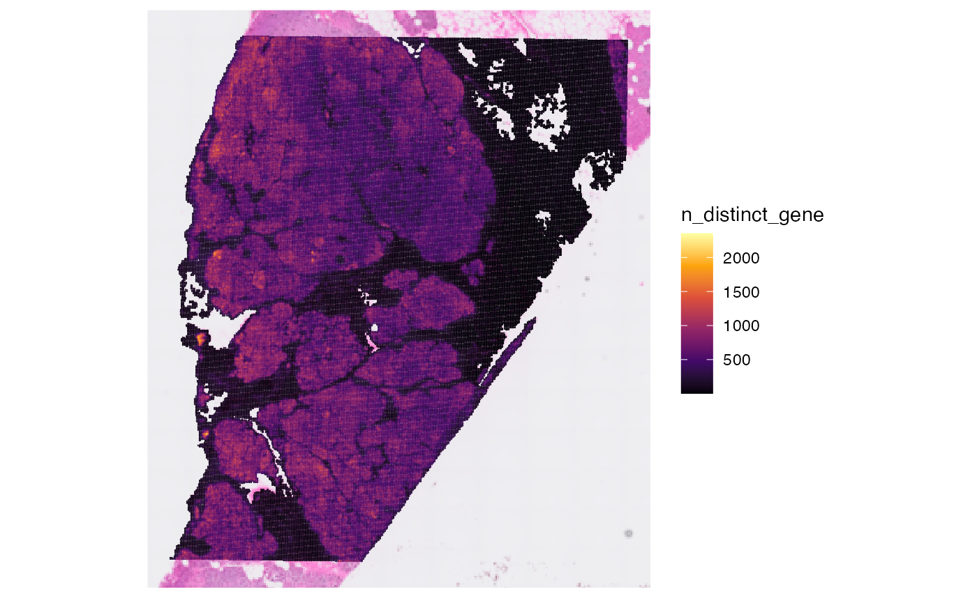
## [1] 106360

Afterwards, you can compute meta data for the observations.

object <- computeMetaFeatures(object)

# plot left
plotSurface(object, color_by = "n_counts_gene")

# plot right
plotSurface(object, color_by = "n_distinct_gene")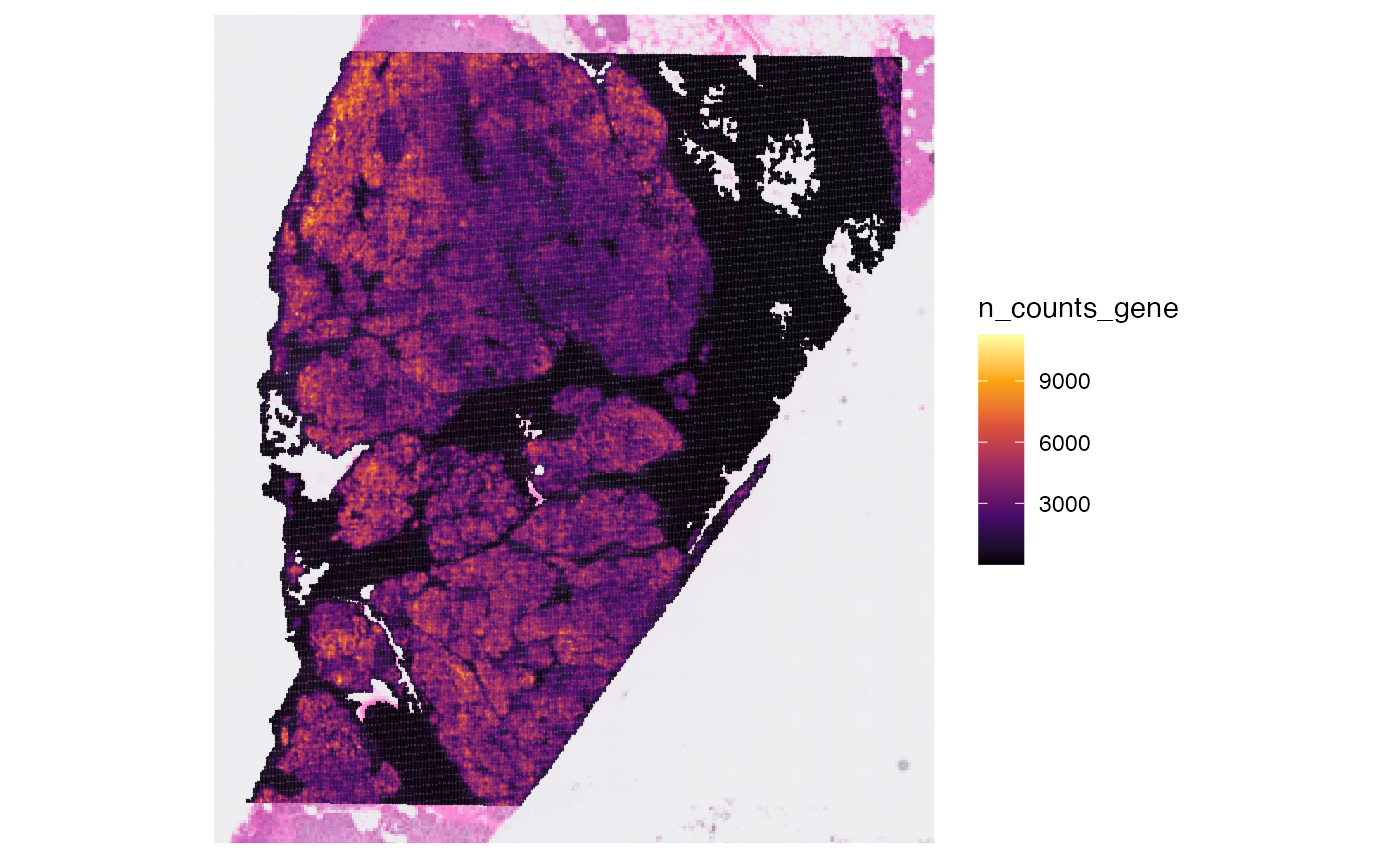

4.2 Matrix processing

The SPATA2 object is initiated with a raw count matrix. For almost all downstream analysis steps it is recommended to use processed matrices. The first step is usually log-normalization. To create a normalized matrix use normalizeCounts(). It uses Seurat::NormalizeData() in the background. The input options for method correspond to the options in this function from the Seurat package. By default, the normalized matrix is named after input for method, activated and thus used by default in downstream analysis and visualization. The function normalizeCounts() can be called multiple times with different inputs for method which populates the list of processed matrices in the respective assay. Furthermore, processed matrices can be added with addProcessedMatrix() if you want to create them with SPATA2-extern functions. The default matrix that is used can be set with activateMatrix(). By default, normalizeCounts() activates the processed matrix it has created.


# obtain matrix names prior to normalization
getMatrixNames(object)
## [1] "counts"

plot_with_raw_counts <- 
  plotSurface(object, color_by = "INS",  pt_clrsp = "Reds 3") + labs(color = "INS\n(Counts)")

# create log normalized matrix
object <- normalizeCounts(object, method = "LogNormalize")

# obtain matrix names after normalization
getMatrixNames(object)
## [1] "counts"       "LogNormalize"

# check active matrix
activeMatrix(object)
## [1] "LogNormalize"

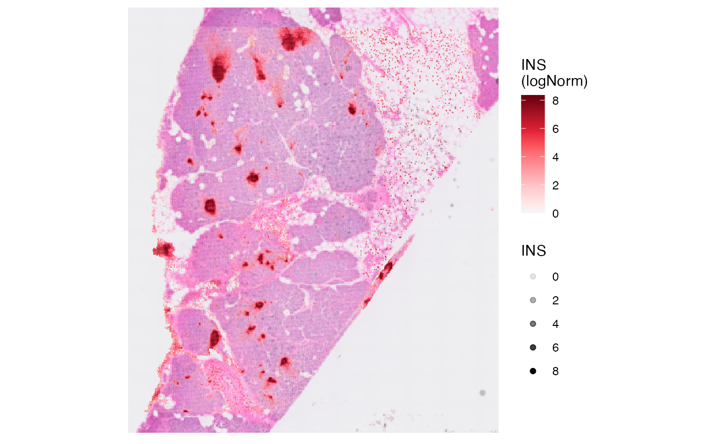
# uses the processed matrix LogNormalize
# use alpha_by to scale transparency to INS as well
plot_with_proc_data <- 
  plotSurface(object, color_by = "INS", alpha_by = "INS", pt_clrsp = "Reds 3") + labs(color = "INS\n(logNorm)") 

# left plot
plot_with_raw_counts

# right plot
plot_with_proc_data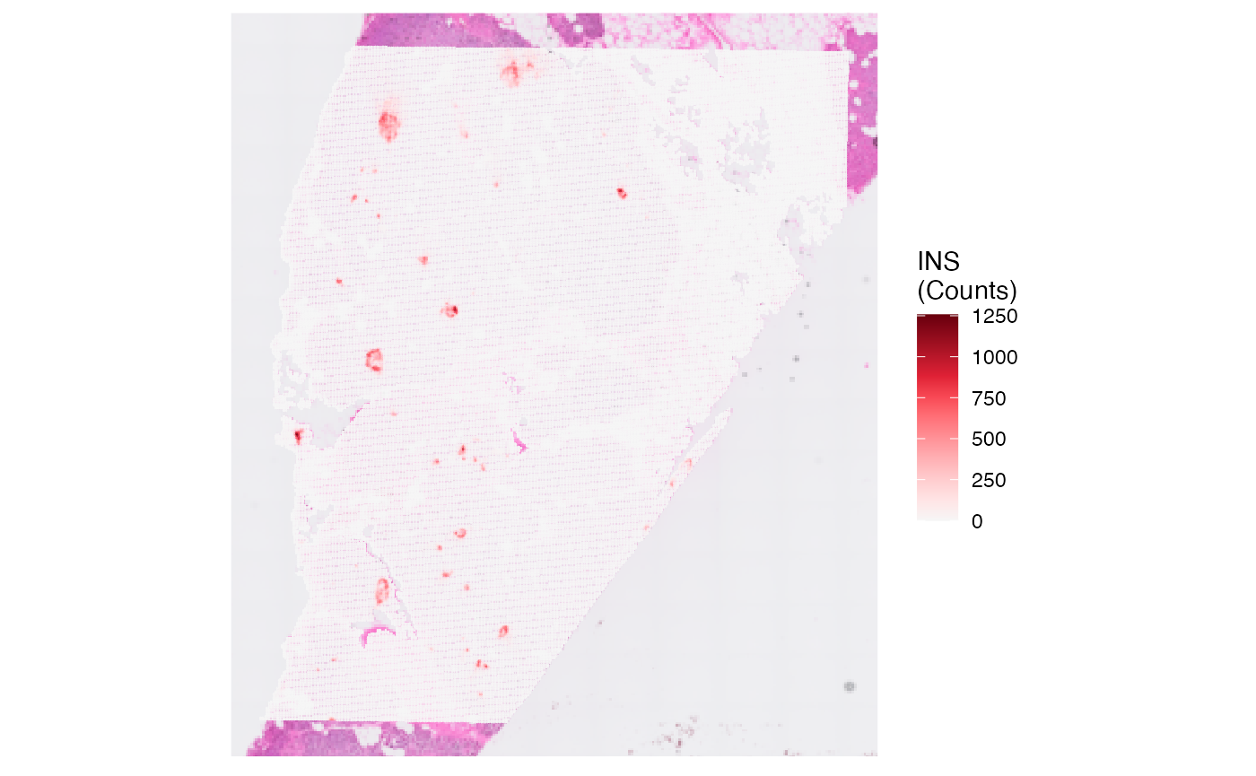

5. Variable genes

Genes of high variability can be identified with wrappers around the some Seurat functions.

# identifies molecules of high variability in the default assay (= gene)
object <- identifyVariableMolecules(object, method = "vst", n_mol = 2500)

var_mols <- getVariableMolecules(object, method = "vst")

str(var_mols)

##  chr [1:2500] "INS" "REG3A" "TTR" "GCG" "GHRL" "SST" "VIP" "PPY" "CARTPT" ...

# example plots
plotSurfaceComparison(object, color_by = var_mols[1:6], pt_clrsp = "Reds 3",  alpha_by = TRUE, nrow = 2)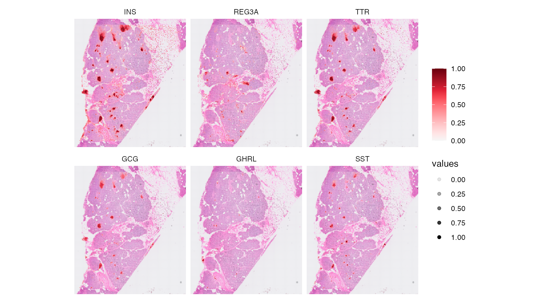

6. Conclusion and more data sets

That’s it. The object can be used for any downstream analyses such as dimensional reduction, clustering, spatial annotation screening or spatial trajectory screening. Refer to tab Tutorials for more links. Furthermore, you can skim our curated data base of spatial data sets for those of platform VisiumHD using SPATAData.

# load package
library(SPATAData)

# filter for samples from platform VisiumHD
sourceDataFrame(platform == "VisiumHD")

## # A tibble: 2 × 18
##   sample_name      donor_species institution lm_source           organ pathology
##   <chr>            <chr>         <chr>       <dttm>              <chr> <chr>    
## 1 HumanLungCancer… Homo sapiens  10X Genomi… 2024-08-04 22:03:33 Lung  tumor    
## 2 HumanPancreasHD  Homo sapiens  10X Genomi… 2024-08-04 22:03:33 Panc… NA       
## # ℹ 12 more variables: platform <chr>, source <chr>, web_link <chr>,
## #   mean_counts <dbl>, median_counts <dbl>, modality_gene <lgl>,
## #   modality_metabolite <lgl>, modality_protein <lgl>, n_obs <int>,
## #   n_tissue_sections <int>, obs_unit <chr>, obj_size <lbstr_by>