Copy Number Variations (CNV) • SPATA2

1. Introduction

InferCNV is used to identify large-scale chromosomal copy number alterations in single cell RNA-Seq data including gains or deletions of chromosomes or large segments of such. Several publications have leveraged this technique. (Patel et al., 2014, Tirosh et al., 2016, Venteicher et al., 2017 )

Note: We are currently encountering problems with the function infercnv:::plot_cnv(). It does not prevent the copy number variation analysis. Sometimes, however, the heatmap is not plotted. Checkout your R console for hints in how far the function did not work properly. We are working on a solution for that. If you encounter warnings raised from runCNV()` let us know.

# load required packages
library(SPATA2)
library(SPATAData)
library(tidyverse)

# load SPATA2 object
object_t313 <- downloadSpataObject(sample_name = "UKF269T")

# alternatively, use diet version (results might differ slightly)
object_t313 <- loadExampleObject(sample_name = "UKF269T")

# only histology
plotSurface(object, = object_t269, pt_alpha = 0)

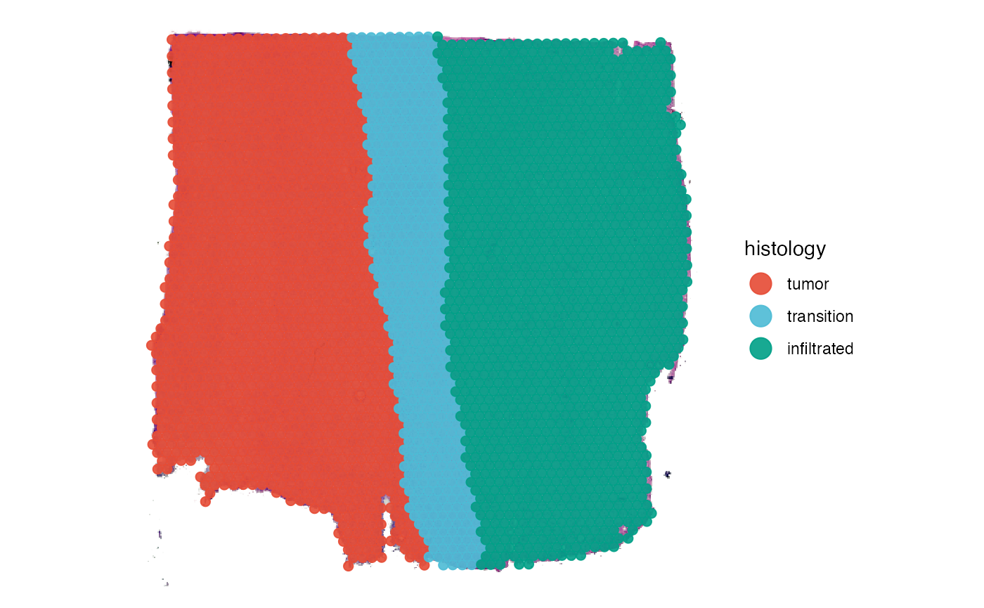
# histological grouping
plotSurface(object = object_t269, color_by = "histology")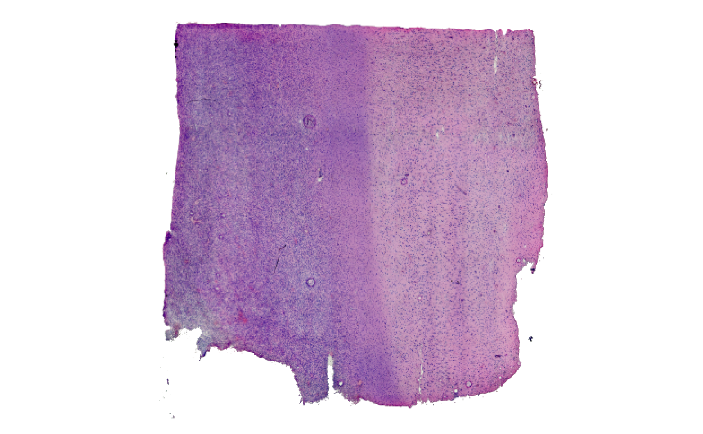

SPATA2 implements the package infercnv published and maintained by Broadinstitute and allows to integrate this technique in your workflow of analyzing spatial trancsriptomic data derived from malignancies.

2. Running CNV Analysis

As with all other functions prefixed with run*() the function runCNV() is a wrapper around all necessary functions needed to conduct copy-number-variation-analysis. The results needed for subsequent analysis steps are stored in the specified SPATA2 object (slot: @cnv). The infercnv-object is stored in the folder specified in the argument directory_cnv_folder.

object_t269 <-
  runCNV(
    object = object_t269,
    # the directory must exist in your file system
    directory_cnv_folder = "data-gbm269/cnv-results", 
    cnv_prefix = "Chr"
    )

If your desired set up deviates from the default you can reach any function of the inferncnv pipeline by entering it’s name as an argument and specify it’s input as a list of arguments with which you want it to be called.

# change input
object_t269 <- 
  runCNV(
    object = object_t269
    directory_cnv_folder = "data-gbm269/cnv-results", 
    clear_noise_via_ref_mean_sd = list(sd_amplifier = 2)
    )

Copy number variation analysis requires reference data. This includes a count matrix from healthy tissue, an annotation file as well as a data.frame that contains information about the chromosome positions. We provide reference data in the list SPATA2::cnv_ref.

names(cnv_ref)

## [1] "annotation" "mtr"        "regions"

summary(cnv_ref)

##            Length   Class      Mode
## annotation        1 data.frame list
## mtr        71067022 dgCMatrix  S4  
## regions           4 data.frame list

runCNV() defaults to the content of this list. The documentation of runCNV() contains a detailed description of the requirements each reference input must meet in order for the function to work.

3. CNV Results

The results are stored in a list inside the SPATA2 object. This list can be obtained via getCnvResults().

cnv_results <- getCnvResults(object_t269)

names(cnv_results)

## [1] "prefix"      "cnv_df"      "cnv_mtr"     "gene_pos_df" "regions_df"

4. Visualization

Note, that the plots below might differ slightly from what you obtain after copy and pasting this code since you are working with a reduced version of the original UKF269T sample. To run this tutorial with the complete data set download sample UKF269T with the SPATAData package.

# if you want the complete object
library(SPATAData)

object <- downloadSpataObject("UKF269T")
object <- runCNV(object)

4.1 Heatmap

The gains and losses of chromosomal segments can be displayed via plotCnvHeatmap(). Without any meta data CNV heatmaps are not that insightful. If you want to visualize the results across certain groups to highlight differences across groups make use of the across and across_subset arguments.

plotCnvHeatmap(object = object_t269, across = "histology", clrp = "npg")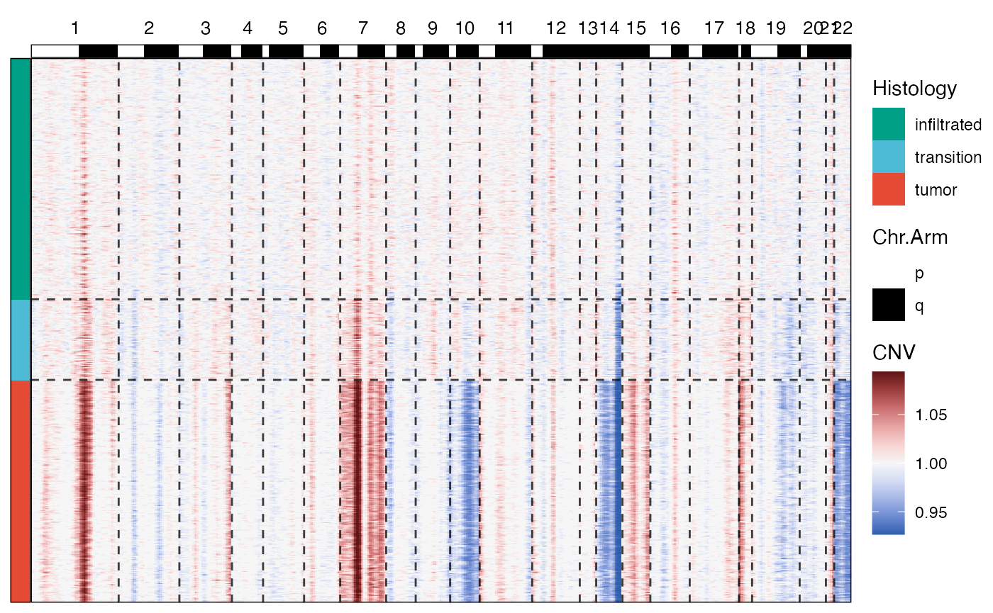

You can add additional meta variables to the legend, numeric and categorical ones alike. Furthermore, you can subset the chromosomes to be displayed as well as the groups across which the results are shown. CNV heatmaps in SPATA2 actually consist of multiple ggplots assembled via the aplot package. You can adjust them by referring to them by name within the ggpLayer argument. For a detailed documentation of how to create the CNV heatmap you desire please refer to the extensive documentation via plotCnvHeatmap().

# a more complex set up
plotCnvHeatmap(
  object = object_t269, 
  across = "histology", 
  across_subset = c("infiltrated", "tumor"), # dont show the transition part
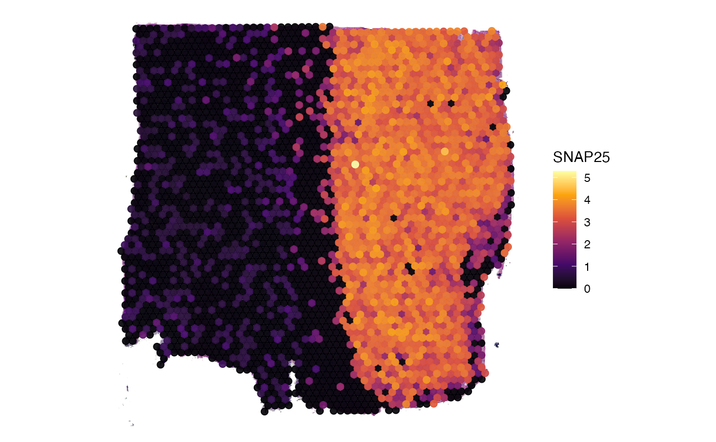
  meta_vars = "SNAP25",  # visualize SNAP25 expression on the left
  meta_vars_clrs = c("SNAP25" = "inferno"), # with the inferno color spectrum 
  chrom_subset = c("1", "3", "7", "10", "14", "15", "18", "22"), # only show these chromosomes
  ggpLayers = list(arm = list(legendNone())) # remove the chrom arm legend
  )

# right plot
plotSurface(object_t269, color_by = "SNAP25", pt_clrsp = "inferno")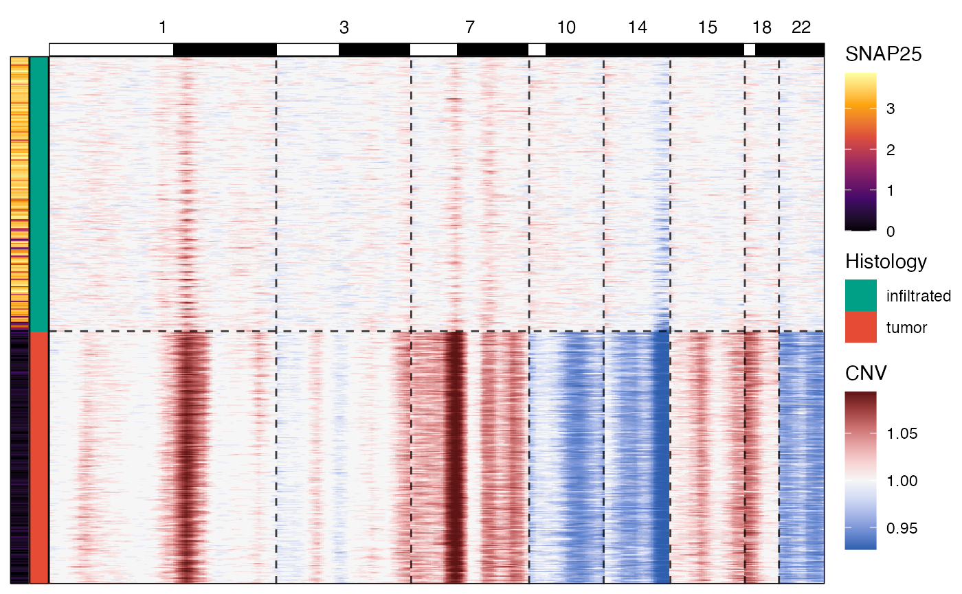

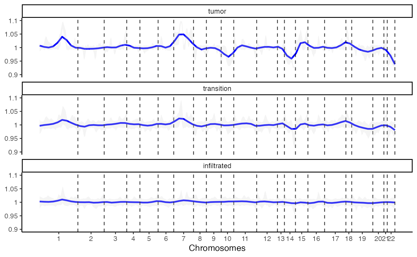
4.2 Lineplot

An additional option to visualize the results provides plotCnvLineplot().

plotCnvLineplot(
  object = object_t269,
  across = "histology", 
  n_bins_bcsp = 1000,
  n_bins_genes = 1000,
  nrow = 3
)

4.3 Surface

The numeric values by which the copy number variations of each chromosome are represented are immediately transferred to the SPATA2 object’s feature data and are thus accessible for all functions that work with numeric variables. The character string specified in argument cnv_prefix combined with the chromosomes number determines the name by which you can refer to these feature variables.

# cnv feature names
getCnvFeatureNames(object = object_t269) %>% head()

## [1] "Chr1" "Chr2" "Chr3" "Chr4" "Chr5" "Chr6"

# are part of all feature names
getFeatureNames(object = object_t269) %>% head()

##            factor           integer           numeric           numeric 
##      "orig.ident"    "nFeature_RNA"      "percent.mt"      "percent.RB" 
##            factor            factor 
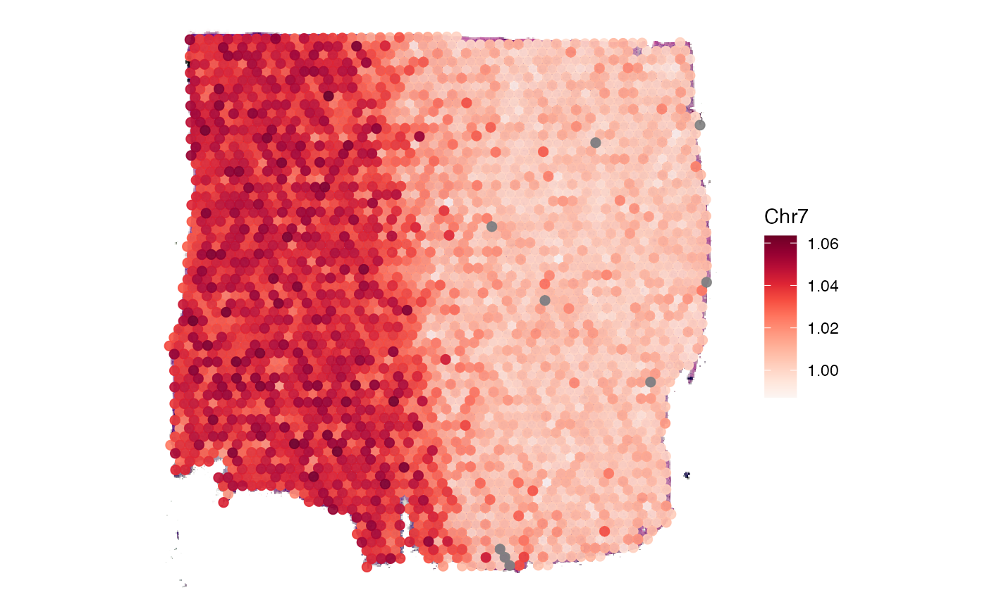
## "RNA_snn_res.0.8"     "bayes_space"

Use plotSurface() to visualize chromosomal alterations directly on the histology.

plotSurface(
  object = object_t269, 
  color_by = "Chr7", 
  pt_clrsp = "Reds"
)

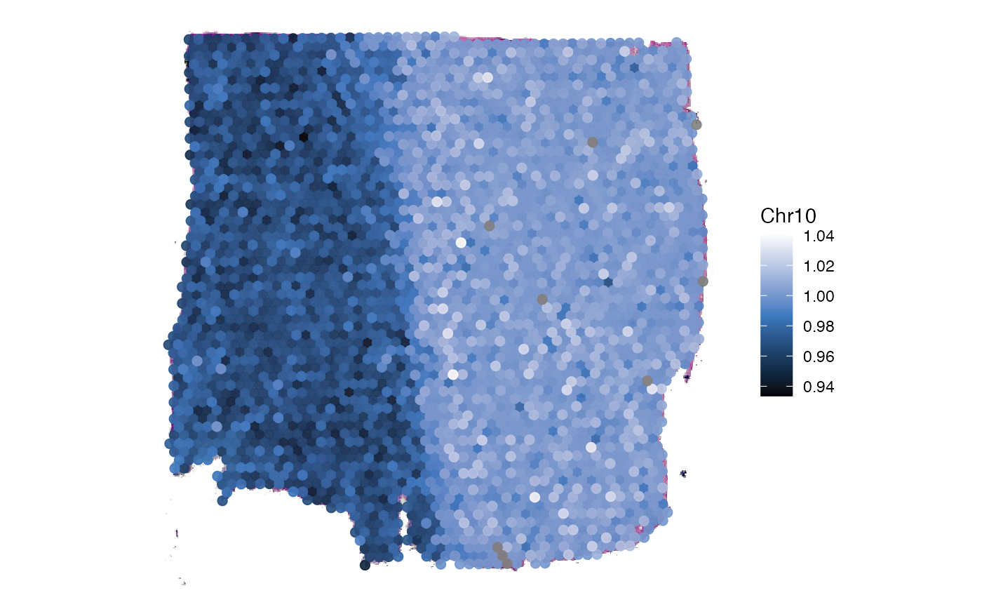
plotSurface(
  object = object_t269, 
  color_by = "Chr10", 
  pt_clrsp = "Oslo" 
)

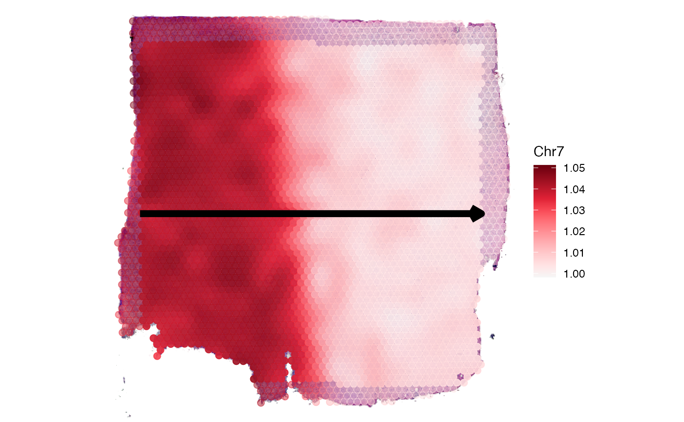
4.4 Gradients

As showcased in our corresponding vignette about spatial trajectories gradients of numeric variables can be displayed. Chromosomal alterations are numeric variables.

plotSpatialTrajectories(
  object = object_t269, 
  ids = "horizontal_mid", 
  color_by = "Chr7", 
  pt_clrsp = "Reds 3"
)

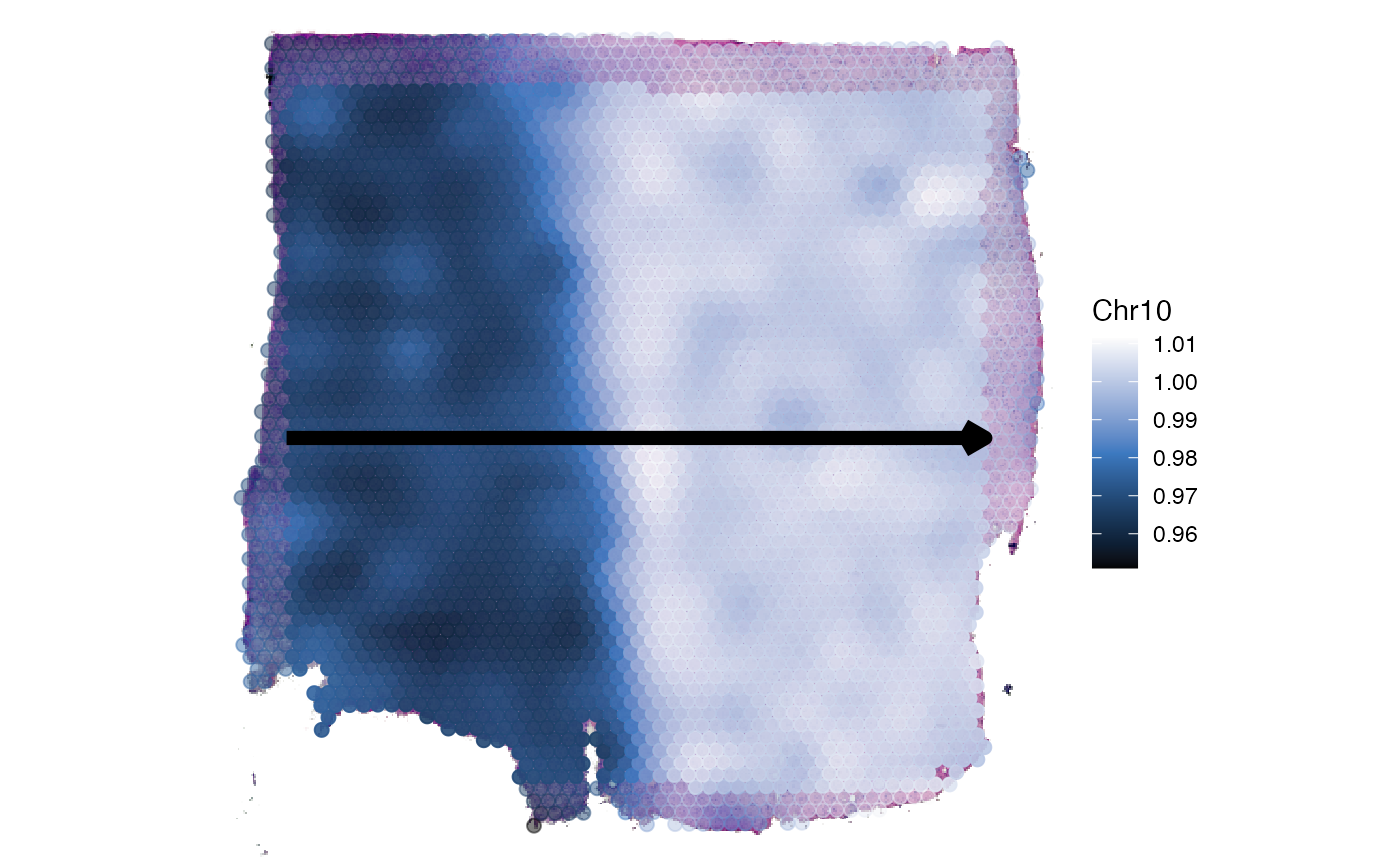
plotSpatialTrajectories(
  object = object_t269, 
  ids = "horizontal_mid", 
  color_by = "Chr10", 
  pt_clrsp = "Oslo"
)

plotStsLineplot(
  object = object_t269, 
  id = "horizontal_mid", 
  variables = "Chr7" 
)

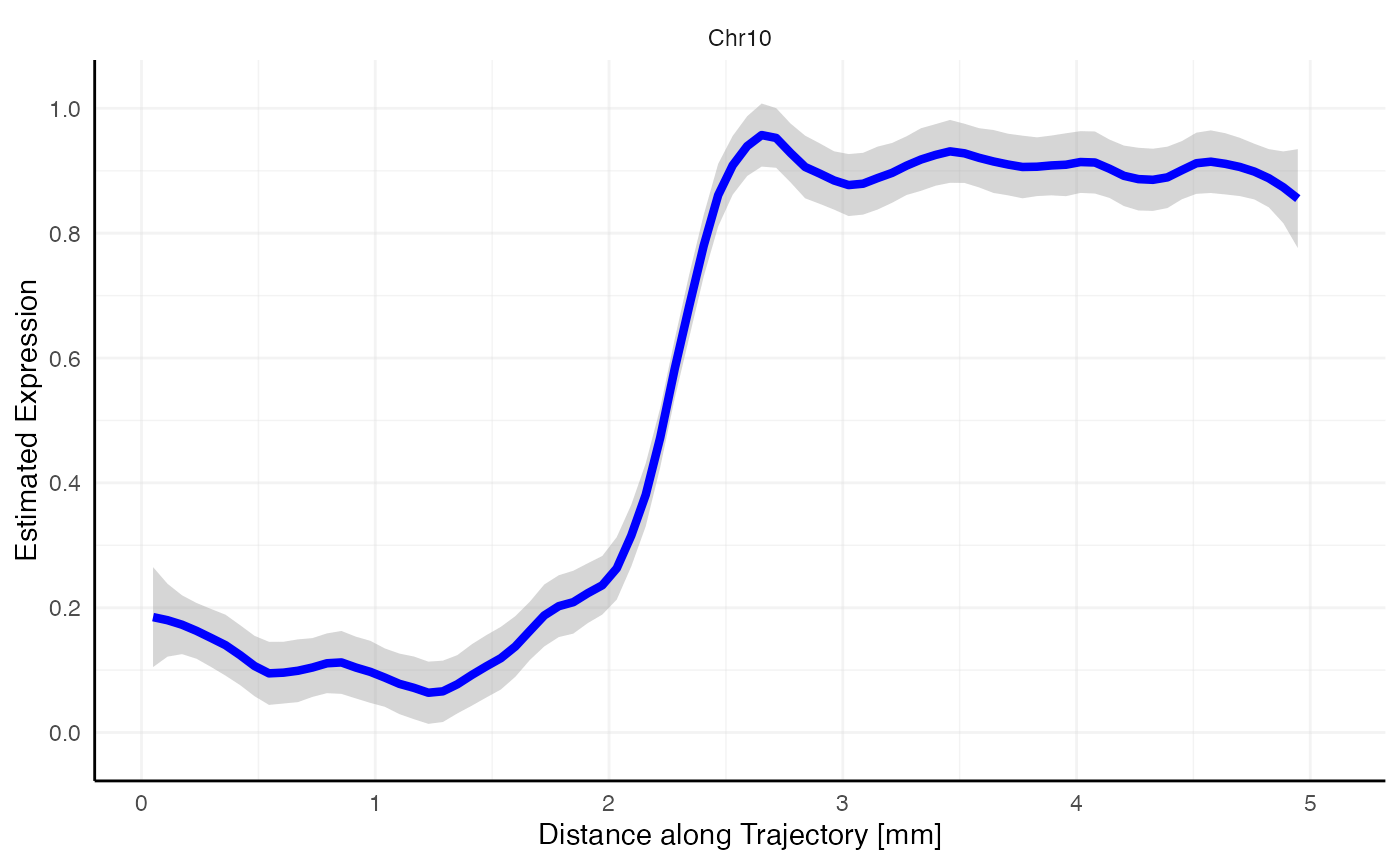
plotStsLineplot(
  object = object_t269, 
  id = "horizontal_mid", 
  variables = "Chr10", 
  line_color = "blue" 
)

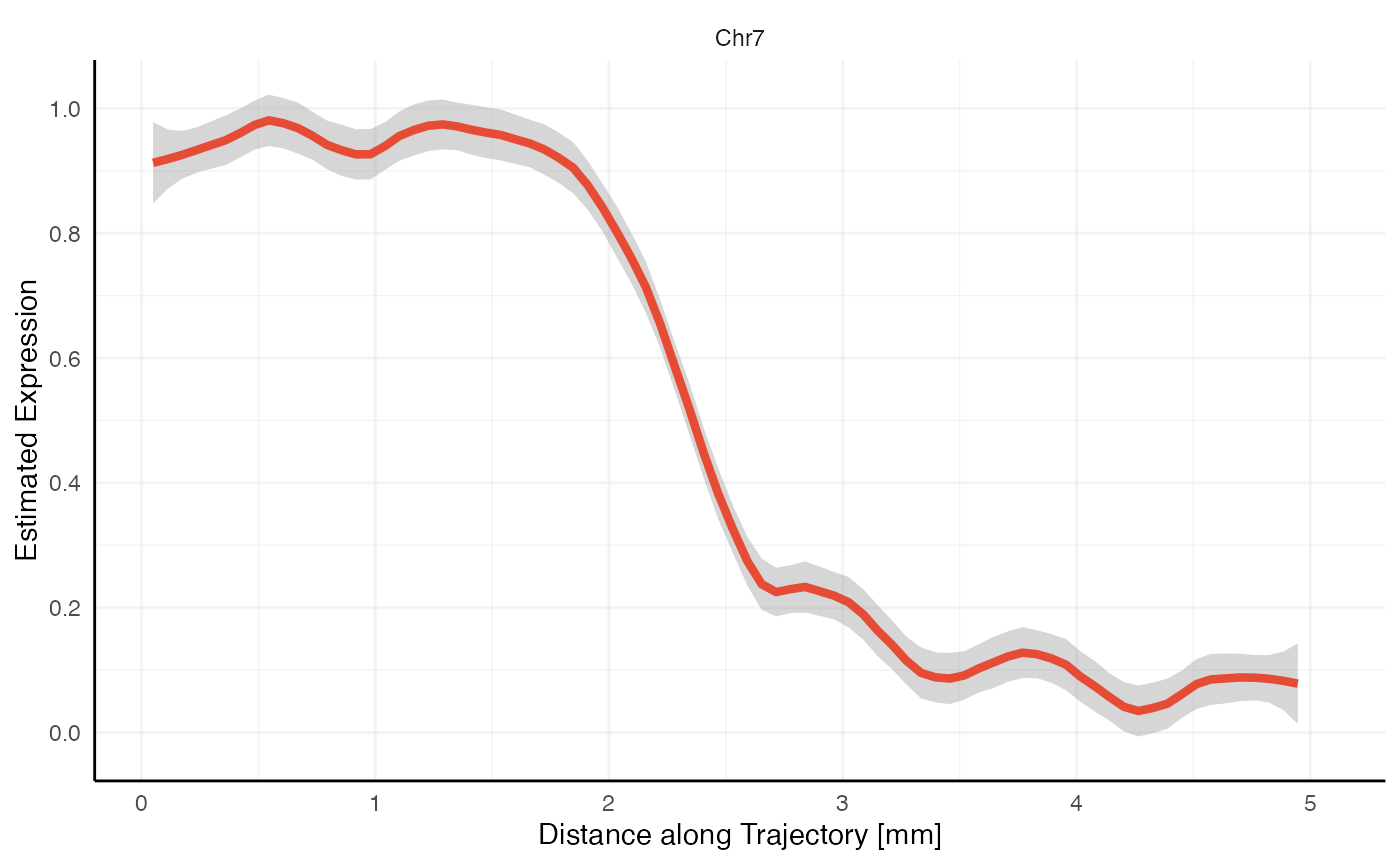
(Note that trajectory lineplots always rescale variables to 0-1 or to low-high.)