Spatial Trajectories
spata-v2-spatial-trajectories.Rmd2. Introduction & overview
With spatial trajectory analysis SPATA2 introduces a new
approach to find, analyze and visualize differently expressed genes and
gene-sets in a spatial context. While the classic differential gene
expression analyzes differences between experimental groups as a whole
it neglects changes of expression levels that can only be seen while
maintaining the spatial dimensions. Spatial trajectories allow to answer
questions that include such a spatial component. E.g.:
- In how far do expression levels change the more we move towards a region of interest?
- Which genes follow the same pattern along these paths?
The spatial trajectory tools provided in SPATA2 enable
new ways of visualization as well as new possibilities to screen for
genes.
As an example we are using a spatial transcriptomic sample of a central nervous system malignancy that features three different, adjacent histological areas: Tumor, a transition zone as well as infiltrated cortex.
library(SPATA2)
library(SPATAData)
library(tidyverse)
library(patchwork)

object_t269 <- downloadSpataObject(sample_name = "269_T")

# load example image annotations
data("image_annotations")

object_t269 <-
  setImageAnnotations(
    object = object_t269,
    img_anns = image_annotations[["269_T"]],
    overwrite = TRUE
  )

# plot results
plotImageGgplot(object = object_t269, frame_by = "coords") +
  ggpLayerThemeCoords()

plotImageAnnotations(
  object = object_t269,
  tags = "hist_example",
  square = TRUE,
  expand = 0.5,
  encircle = FALSE,
  nrow = 2,
  display_caption = FALSE
)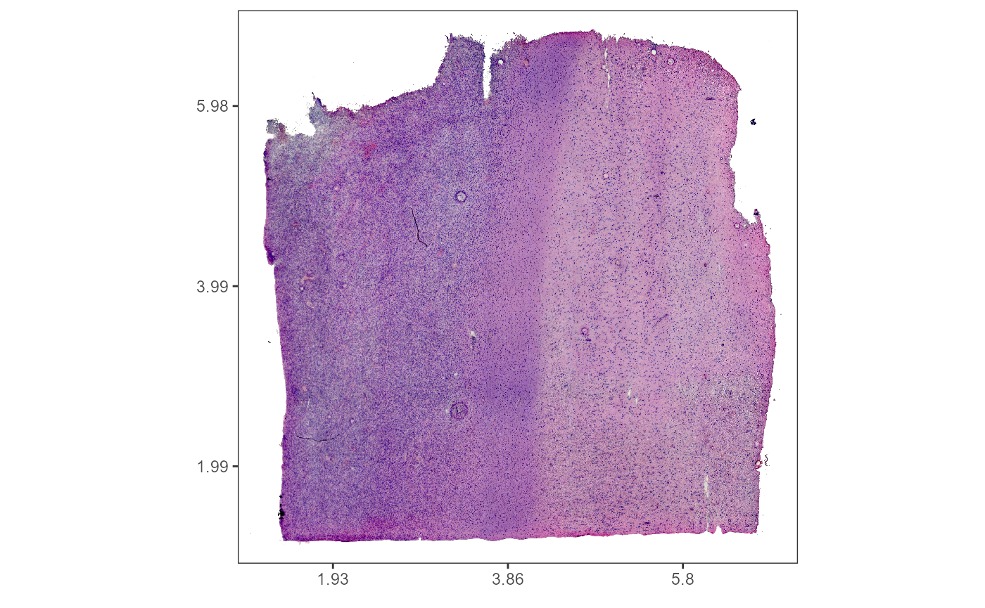
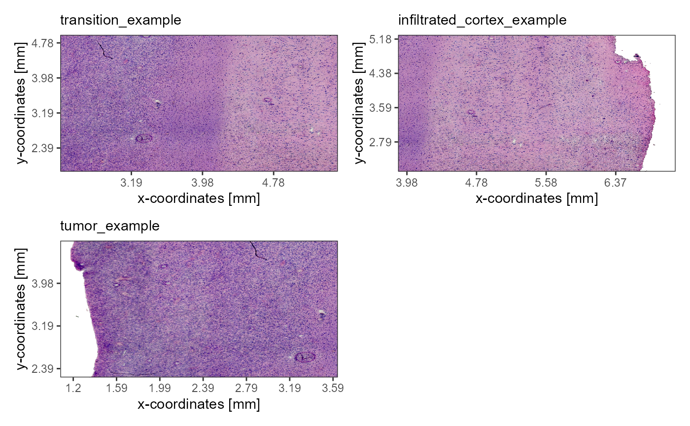
Fig.1 Example sample T269.
3. Set up spatial trajectories
Spatial trajectories can be added to the spata2 object
via two functions, namely createSpatialTrajectory() and
addSpatialTrajectory().
3.1 Interactive drawing
Fig.2 shows the interface of
createSpatialTrajectories(). To draw a trajectory double
click on the surface plot to mark the trajectory’s starting point and
then double click again to mark the endpoint. The result should look
somewhat like the trajectory drawn in Fig.2.
object_t269 <- createSpatialTrajectories(object = object_t269)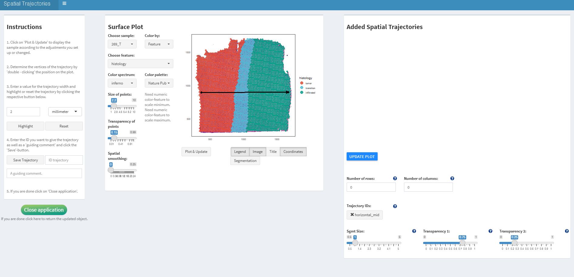
Fig.2 Interface of createSpatialTrajectories() with a drawn trajectory.
If you are satisfied with the course of the trajectory determine the width of the trajectory’s scope on the left and click on highlight. Then enter a valid ID with which you want to name the trajectory and click on ‘Save Trajectory’.

Fig.3 Adjust trajectory width, higlight the spots and enter a name.
The trajectory should appear on the right side of the interface under ‘Trajectory IDs:’. Click on the name and click on ‘UPDATE PLOT’ to visualize the trajectory with the barcode-spots it includes on the histology image.
3.2 With code
Instead of drawing the spatial trajectory you can add it directly by
explicitly naming its course via start- and endpoint using the function
addSpatialTrajectory().
object_t269 <-
  addSpatialTrajectory(
    object = object_t269,
    id = "horizontal_mid",
    start = c("1.5mm", "3.5mm") ,
    end = c("6.5mm", "3.5mm") ,
    width = "2mm",
    overwrite = TRUE
  )
4. Extract trajectory information
Spatial trajectories are stored in form of S4 objects of class
SpatialTrajectory. The can be extracted via
getSpatialTrajectory().
traj_ids <- getSpatialTrajectoryIds(object = object_t269)

traj_ids
## [1] "horizontal_mid"
traj_obj <- getSpatialTrajectory(object = object_t269, id = "horizontal_mid")

traj_obj
## An object of class "SpatialTrajectory"
## Slot "coords":
## # A tibble: 3,213 x 6
## barcodes sample x y section outline
## <chr> <chr> <dbl> <dbl> <chr> <lgl>
## 1 AAACAAGTATCTCCCA-1 269_T 1450. 731. 1 FALSE
## 2 AAACACCAATAACTGC-1 269_T 411. 547. 1 FALSE
## 3 AAACAGAGCGACTCCT-1 269_T 1359. 1516 1 FALSE
## 4 AAACATTTCCCGGATT-1 269_T 1386. 493. 1 FALSE
## 5 AAACCCGAACGAAATC-1 269_T 1614. 838. 1 FALSE
## 6 AAACCGGGTAGGTACC-1 269_T 527. 916. 1 FALSE
## 7 AAACCGTTCGTCCAGG-1 269_T 700. 696 1 FALSE
## 8 AAACCTAAGCAGCCGG-1 269_T 1210. 408. 1 FALSE
## 9 AAACCTCATGAAGTTG-1 269_T 416. 1026. 1 FALSE
## 10 AAACGAGACGGTTGAT-1 269_T 1167. 1061. 1 FALSE
## # i 3,203 more rows
##
## Slot "info":
## $current_dim
## [1] 1939 2000 3
##
## $current_just
## $current_just$angle
## [1] 0
##
## $current_just$flipped
## $current_just$flipped$horizontal
## [1] FALSE
##
## $current_just$flipped$vertical
## [1] FALSE
##
##
##
##
## Slot "width_unit":
## [1] "mm"
##
## Slot "comment":
## [1] ""
##
## Slot "id":
## [1] "horizontal_mid"
##
## Slot "projection":
## # A tibble: 2,301 x 6
## barcodes sample x y projection_length trajectory_part
## <chr> <chr> <dbl> <dbl> <dbl> <chr>
## 1 GCAACACACTAGAACT-1 269_T 377. 830 0.0397 Part 1
## 2 TCAACATCGACCGAGA-1 269_T 377. 874. 0.439 Part 1
## 3 TGCAGCTACGTACTTC-1 269_T 377. 917. 0.839 Part 1
## 4 TTCAGGCGTCAAAGCC-1 269_T 378. 961. 1.24 Part 1
## 5 GGGCCCTACGAAAGGG-1 269_T 378. 1004 1.64 Part 1
## 6 TACTCGGCACGCCGGG-1 269_T 379. 1048. 2.44 Part 1
## 7 TTACTATCGGCTTCTC-1 269_T 379. 1091. 2.84 Part 1
## 8 CTGATAGTGTATCTCA-1 269_T 380. 1135. 3.24 Part 1
## 9 AATGGTCCACCGTTCA-1 269_T 380. 1178. 3.64 Part 1
## 10 TAACAATATTTGTTGC-1 269_T 381. 1222. 4.04 Part 1
## # i 2,291 more rows
##
## Slot "sample":
## [1] "269_T"
##
## Slot "segment":
## x y xend yend part
## 1 376.5661 878.6542 1631.786 878.6542 part_1
##
## Slot "width":
## [1] 502.0881For more information on the S4 class use
?SpatialTrajectory.
5. Visualization with spatial trajectories
Spatial trajectories indicate a direction, in case of horizontal_mid it indicates the direction from left to right or from tumor to infiltrated cortex. This can be used to infer and visualize gene expression changes in space.
5.1 Numeric variables
The four genes EGFR, MBP, SNAP25 and BCL9 serve as an example. They first three are marker genes detected by DEA based on the histological grouping.
genes <- c("EGFR", "MBP", "SNAP25", "BCL9")

gene_colors <- color_vector(clrp = "npg", names = genes)

gene_colors
## EGFR MBP SNAP25 BCL9
## "#E64B35FF" "#4DBBD5FF" "#00A087FF" "#3C5488FF"
trajectory <-
  ggpLayerTrajectories(
    object = object_t269,
    ids = "horizontal_mid",
    size = 1
    )

tissue_outline <- ggpLayerTissueOutline(object = object_t269)

plist <-
  imap(
    .x = gene_colors,
    .f = function(color, gene){

      plotSurface(object_t269, color_by = gene, display_image = F) +
        scale_color_gradient(low = alpha("white", 0), high = color) +
        tissue_outline +
        trajectory

    })

wrap_plots(plist, ncol = 2)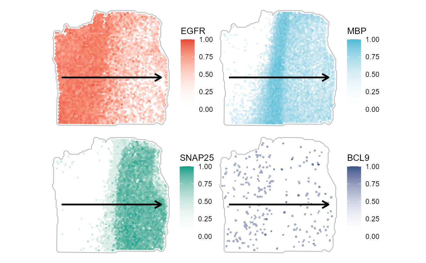
Fig.4 Surface plots with trajectory course.
The inferred expression changes along the trajectory can be plotted via line plots…
plotTrajectoryLineplot(
  object = object_t269,
  id = "horizontal_mid",
  variables = genes,
  smooth_se = TRUE,
  clrp_adjust = gene_colors
) 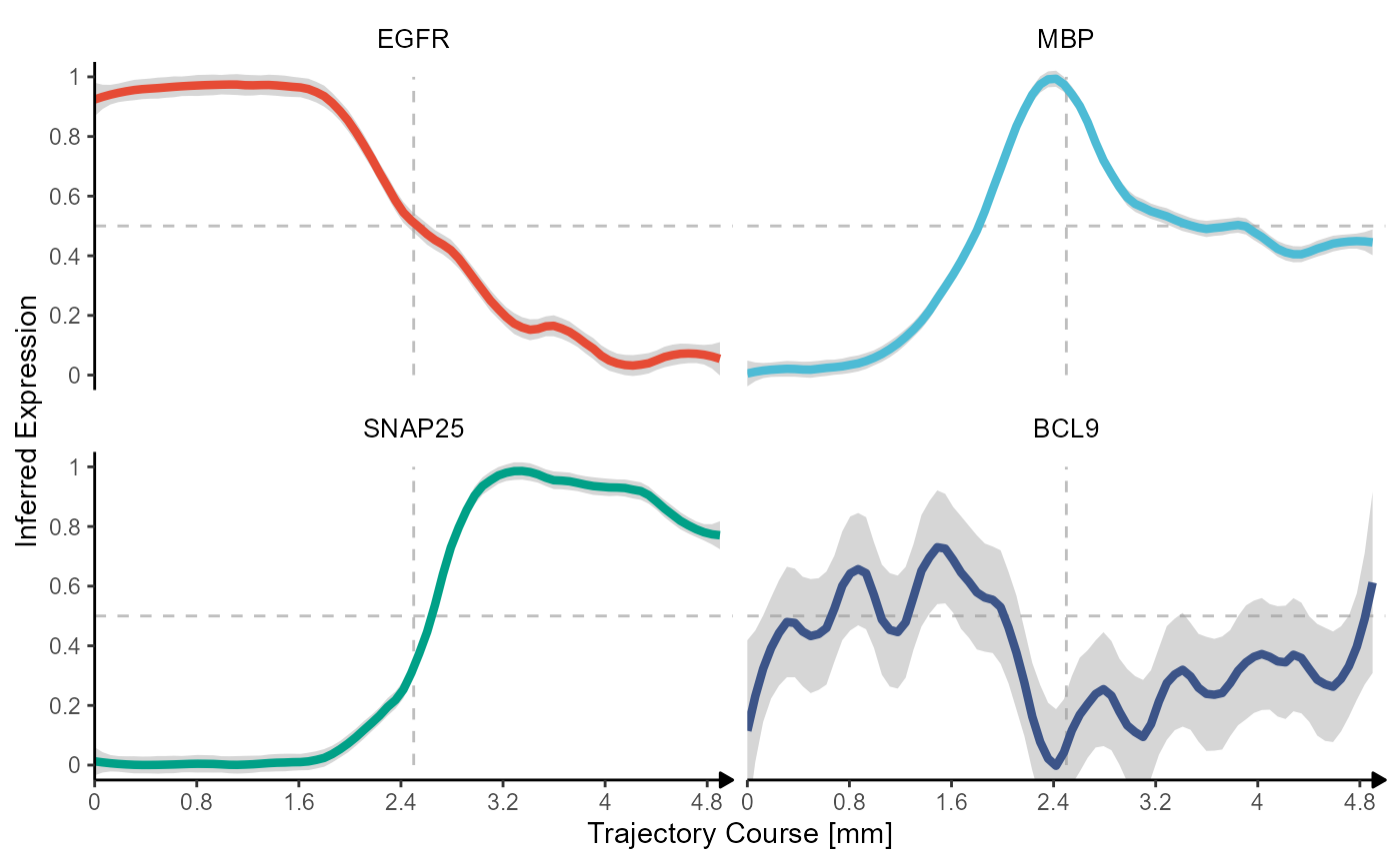
Fig.5 Inferred gene expression along the trajectory with line plots.
… or ridgeplots.
plotTrajectoryRidgeplot(
  object = object_t269,
  id = "horizontal_mid",
  variables = genes,
  clrp_adjust = gene_colors
) + legendNone()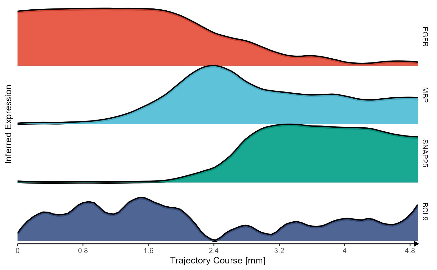
Fig.6 Inferred gene expression along trajectory with ridgeplots.
5.2 Grouping variables
The changes of grouping variables along the trajectory can not be displayed with line plots but with bar plots
# load example list
data("spatial_segmentations")

object_t269 <-
  addFeatures(
    object = object_t269,
    feature_df = spatial_segmentations[["269_T"]],
    overwrite = TRUE
  )

# surface
hist_plot_surface <-
  plotSurface(
    object = object_t269,
    color_by = "histology",
    pt_clrp = "npg"
    )

seurat_plot_surface <-
  plotSurface(
    object = object_t269,
    color_by = "seurat_clusters",
    pt_clrp = "lo"
  )

# bar plots
hist_barplot <-
  plotTrajectoryBarplot(
    object = object_t269,
    id = "horizontal_mid",
    grouping_variable = "histology",
    clrp = "npg"
  )

seurat_barplot <-
  plotTrajectoryBarplot(
    object = object_t269,
    id = "horizontal_mid",
    grouping_variable = "seurat_clusters",
    clrp = "lo"
  )

# plot results
hist_plot_surface + trajectory

hist_barplot

seurat_plot_surface + trajectory

seurat_barplot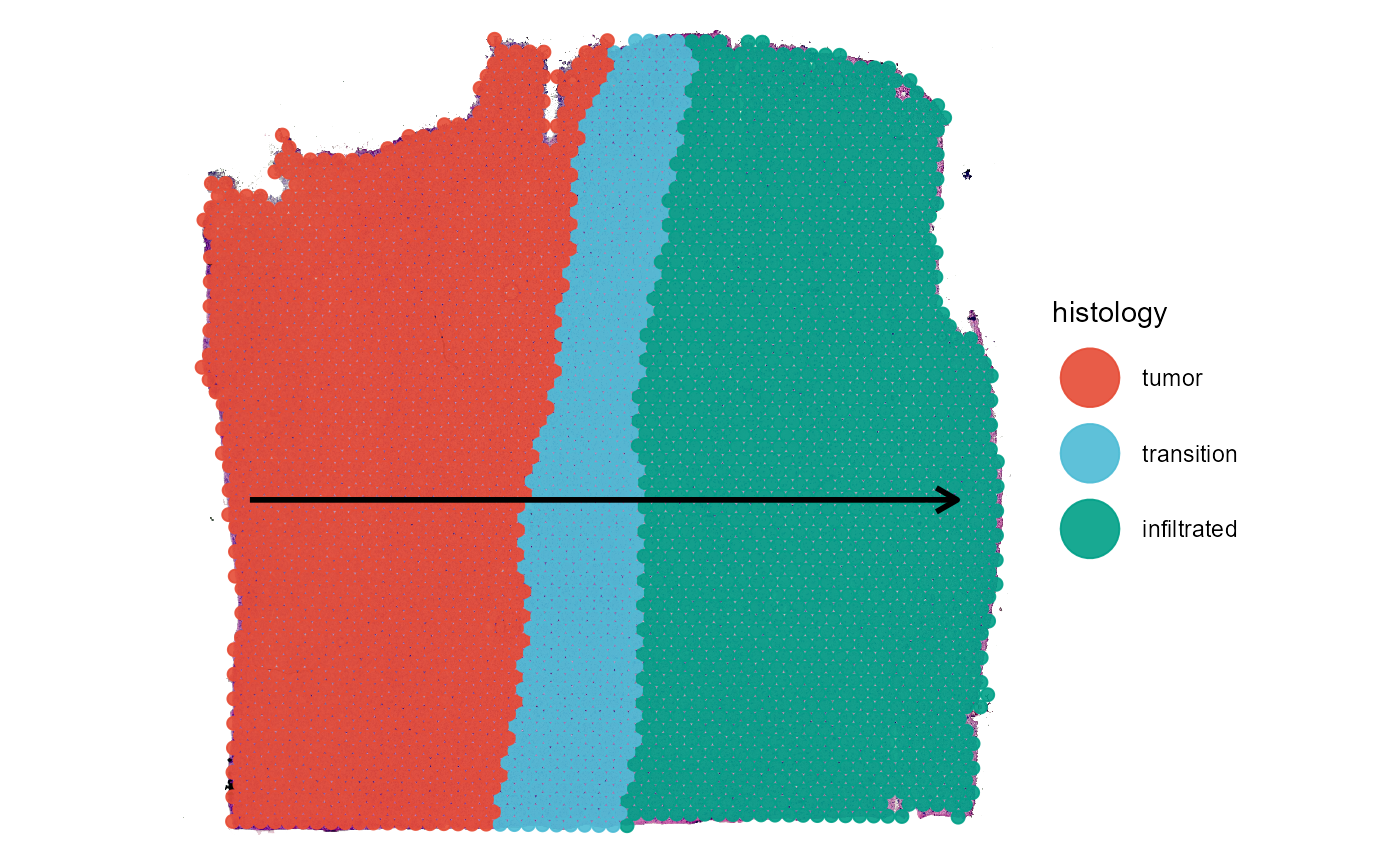
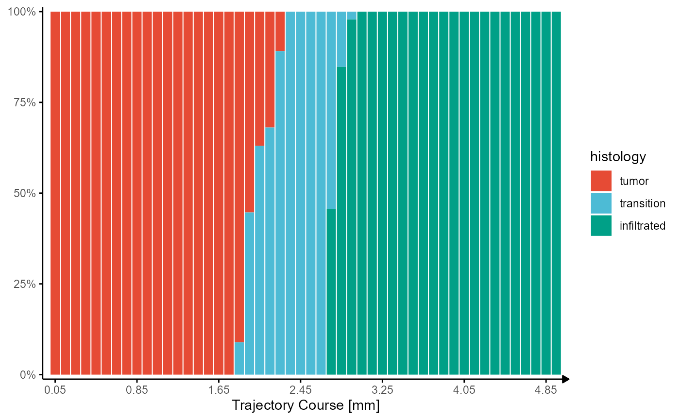
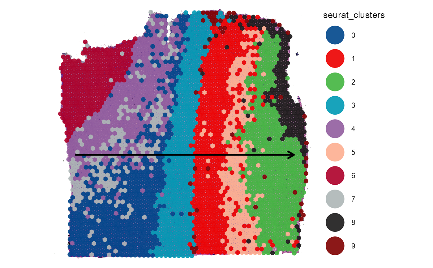
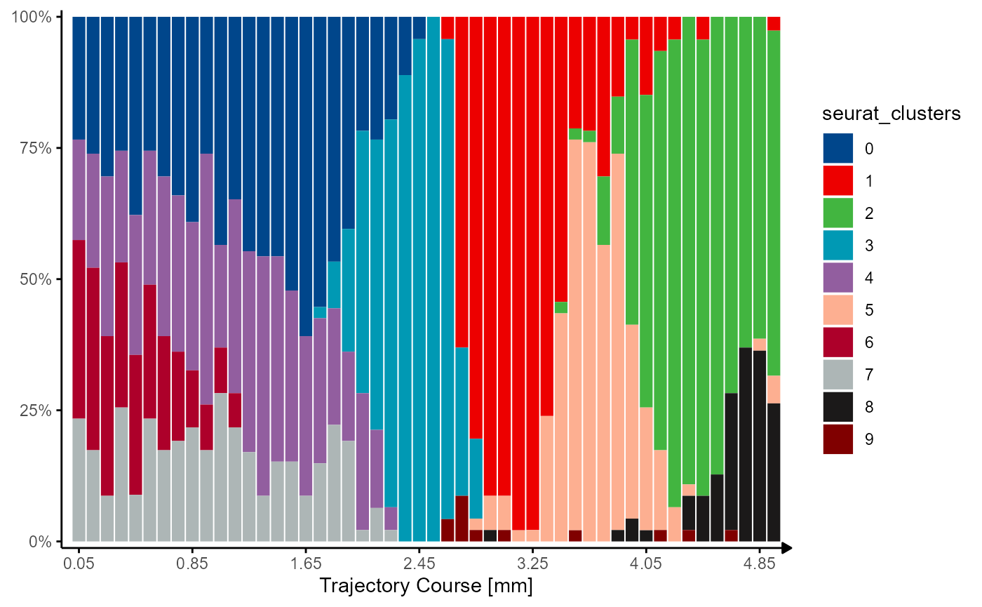
Fig.7 Visualizing grouping variables.