Clustering

1. Prerequisites

None.

2. Introduction

Grouping variables divide the barcode-spots of sample into groups whose properties can be compared against each other. For instance, the grouping of barcode-spots can be the result of clustering algorithms or manual spatial segmentation. This tutorial shows how to apply and add clustering in SPATA2.

library(tidyverse)
library(SPATA2)
library(SPATAData)

object_t275 <- downloadSpataObject(sample_name = "275_T")

plotImageGgplot(object = object_t275)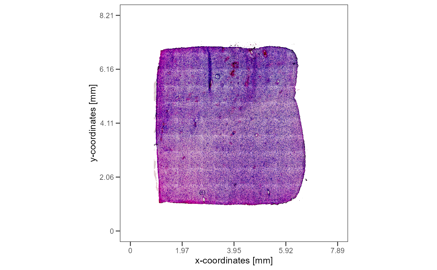

Fig.1 The example sample.

3. Clustering

There are several algorithms out there that can be used to divide your sample into subgroups. While initiateSpataObject_10X() integrates the clustering algorithm used by the Seurat-package there are actually many more. As the use of clustering is highly depending on the biological question it makes sense to use several approaches and algorithms.

3.1 Clustering within SPATA2

SPATA2 provides wrappers around several clustering algorithms. Cluster algorithms that add their results immediately to the SPATA2 object are prefixed with with run-* and suffixed with *-Clustering(). E.g. runBayesSpaceClustering() or runSeuratClustering().

# current grouping options
getGroupingOptions(object_t275)

##            factor            factor            factor 
##             "snn"     "bayes_space" "seurat_clusters"

Argument name specifies the name of the output grouping variable.

# run the pipeline
object_t275 <- 
  runBayesSpaceClustering(
    object = object_t275, 
    name = "bayes_space" # the name of the output grouping variable
  )

# results are immediately stored in the objects feature data
getGroupingOptions(object_t275)

##            factor            factor            factor 
##             "snn" "seurat_clusters"     "bayes_space"

Input of argument name sets the name of the grouping variable.

plotSurface(
  object = object_t275, 
  color_by = "bayes_space", 
  pt_clrp = "uc"
)

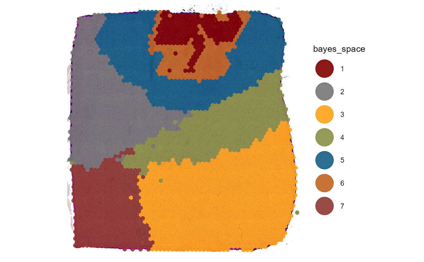
Fig.2 BayesSpace clustering results.

3.2 Clustering outside of SPATA2

Clustering can result from a multitude of cluster algorithms. If they are not implemented in SPATA2 functions you can add them using the addFeatures() function.

kmeans_res <- 
  stats::kmeans(
    x = getPcaMtr(object_t275), 
    centers = 7, 
    algorithm = "Hartigan-Wong"
  )

head(kmeans_res[["cluster"]])

## AAACAAGTATCTCCCA-1 AAACACCAATAACTGC-1 AAACAGAGCGACTCCT-1 AAACAGCTTTCAGAAG-1 
##                  5                  7                  1                  3 
## AAACAGGGTCTATATT-1 AAACAGTGTTCCTGGG-1 
##                  2                  2

cluster_df <- 
  as.data.frame(kmeans_res[["cluster"]]) %>% 
  tibble::rownames_to_column(var = "barcodes") %>% 
  magrittr::set_colnames(value = c("barcodes", "kmeans_4_HW")) %>% 
  tibble::as_tibble()

cluster_df[["kmeans_4_HW"]] <- as.factor(cluster_df[["kmeans_4_HW"]])

cluster_df

## # A tibble: 3,734 x 2
##    barcodes           kmeans_4_HW
##    <chr>              <fct>      
##  1 AAACAAGTATCTCCCA-1 5          
##  2 AAACACCAATAACTGC-1 7          
##  3 AAACAGAGCGACTCCT-1 1          
##  4 AAACAGCTTTCAGAAG-1 3          
##  5 AAACAGGGTCTATATT-1 2          
##  6 AAACAGTGTTCCTGGG-1 2          
##  7 AAACATTTCCCGGATT-1 2          
##  8 AAACCGGGTAGGTACC-1 3          
##  9 AAACCGTTCGTCCAGG-1 2          
## 10 AAACCTAAGCAGCCGG-1 2          
## # i 3,724 more rows

Only requirement is a barcodes variable to map the groups to the barcode-spots. Note that a variable must be of class factor in order to be recognized as a grouping variable.

# feature names before adding
getGroupingOptions(object_t275)

##            factor            factor            factor 
##             "snn" "seurat_clusters"     "bayes_space"

# add the cluster results
object_t275 <- 
  addFeatures(
    object = object_t275,
    feature_df = cluster_df
    )

# feature names afterwards
getGroupingOptions(object_t275)

##            factor            factor            factor            factor 
##             "snn" "seurat_clusters"     "bayes_space"     "kmeans_4_HW"

Continue by visualizing your results or by investigating their transcriptional characteristics using differentially expressed analysis (DEA)).

plotSurface(
  object = object_t275,
  color_by = "kmeans_4_HW",
  pt_clrp = "jama"
  ) +
  labs(color = "Kmeans HW")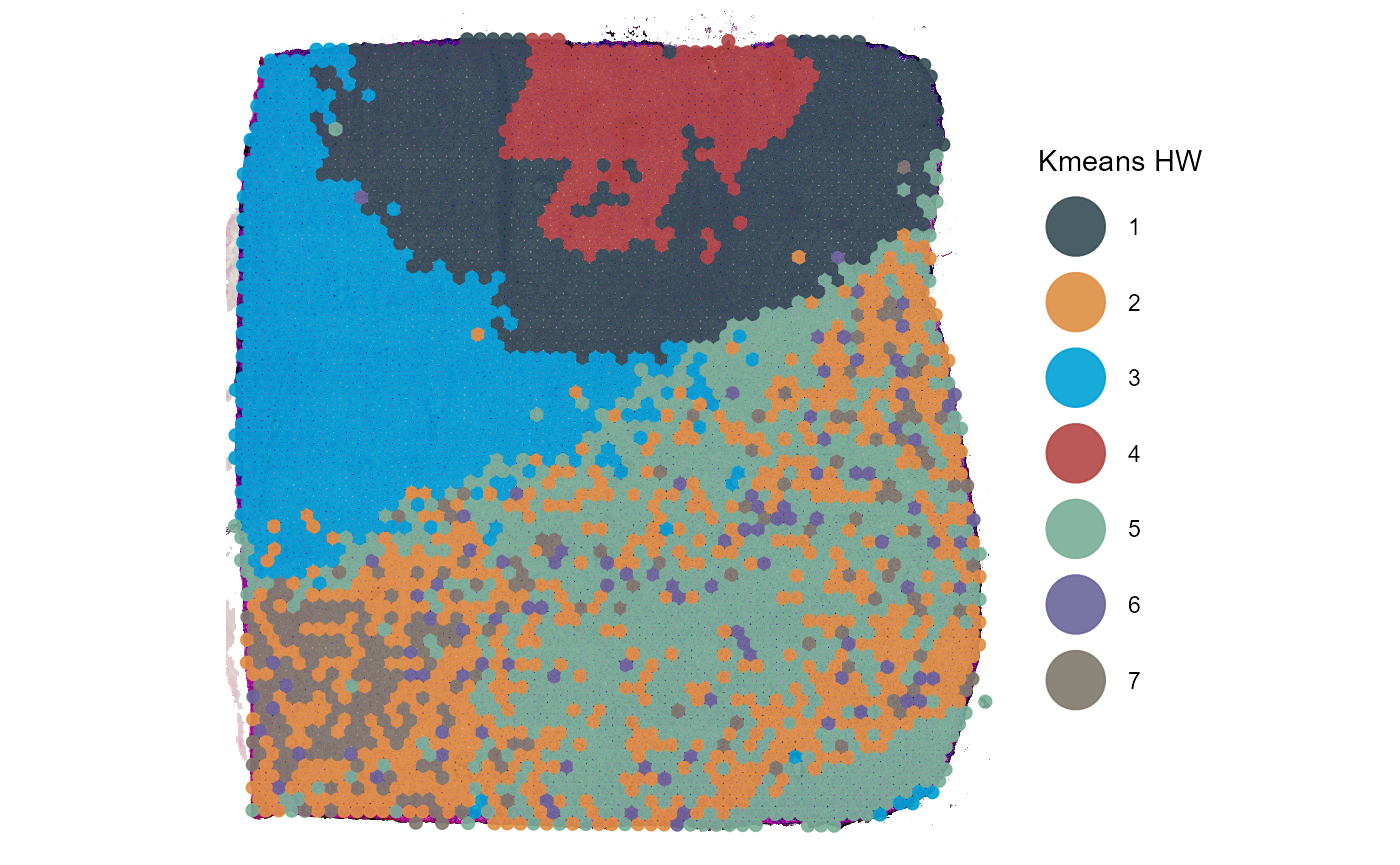

Fig.3 Leiden clustering results