Image Annotations

1. Prerequisites

Please make sure to be familiar with the following vignettes before reading this tutorial.

Spatial Segmentation vs. Image Annotations

2. Introduction & overview

This tutorial describes how to use SPATA to integrate the histology of your sample into your analysis.

library(SPATA2)
library(SPATAData)
library(tidyverse)

object_t313 <- SPATAData::downloadSpataObject(sample_name = "313_T", file = NULL)

3. The HE-image

The HE-image of your spatial sample is stored in slot @images of the spata2 object. Sample T313 is a glioblastoma with a prominent necrotic area in it’s center.

plotImageGgplot(object_t313)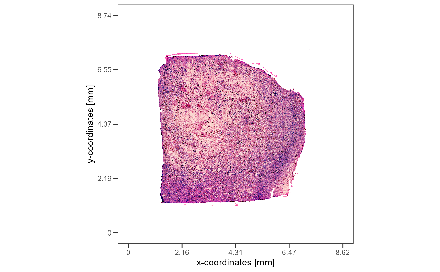

Fig.1 The HE-image.

To analyze the necrotic area we’ll use SPATA2 image annotation system.

3. Creating image annotations

Image annotations are structures in histology image whose spatial extent is captured in form of a polygon and saved in the spata2 object. For more details on how this is translated into R-code see below. To add image annotations to the spata2 object you can make use of the function createImageAnnotations(). This function lets you access an interactive application in which you can encircle the structure or area you want to annotate.

# interactively
object <- createImageAnnotations(object = object_t313)

# or manually 
data("image_annotations")

object <- 
  setImageAnnotation(
    object = object_t313,
    img_ann = image_annotations$`313_T`[["necrotic_center"]], 
    overwrite = TRUE
    )

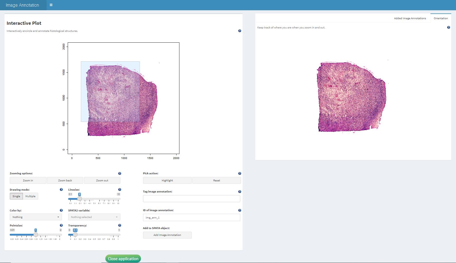
Fig.2 The interface of createImageAnnotations()

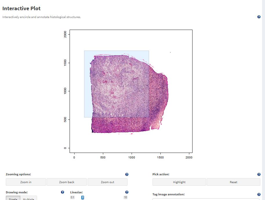
Fig.3 Zooming options allow to inspect the HE-image in detail.

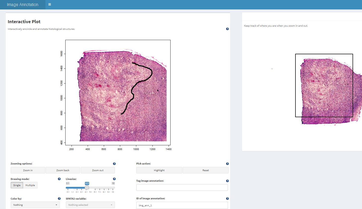
Fig.4 Encircling the area of interest.

The left plot Interaction is where the magic happens. The right plot is used for orientation if you want to zoom in and out. Double click on the left image to start the drawing process. Double click again to stop drawing. If you are using drawing mode Single click on ‘Highlight’ to highlight the encircled area, enter the tags you want to tag the annotation with, enter the ID with which you want to name the annotation and click on ‘Add Image Annotation’. If you are in drawing mode Multiple stopping the drawing immediately highlights the encircled area. This allows to quickly encircle multiple structures of the same kind that are tagged with the same tags (e.g. multiple small vessel). The tab on the right called ‘Added Image Annotations’ allows to visualize all image annotations saved so far.

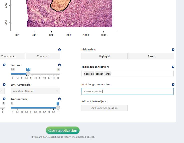
Fig.5 Area is encircled and can be added as an image annotation.

Make sure to click on ‘Close application’ to return the spata2 object containing the results.

4. Visualizing image annotations

To visualize the structures you have annotated use plotImageAnnotations().

plotImageAnnotations(
  object = object_t313,
  ids = "necrotic_center",
  expand = 0.5,
  square = TRUE
  )

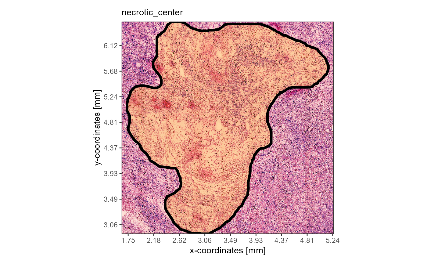
Fig.6 Simple visualization of image annotations.

The function ggpLayerImgAnnOutline() creates an additional layer that can be added to other surface plots created with ggplot2. This is useful if you want to visualize the extent of certain histological structures in relation to certain features or gene expression.

# ggpLayer*functions create standalone ggproto objects 
# that can be used to customize other ggplots
layer_necrotic <- 
  ggpLayerImgAnnOutline(
    object = object_t313, 
    ids = "necrotic_center",
    fill = "gray", 
    alpha = 0.5
    )

plotSurface(
  object = object_t313, 
  color_by = "nCount_Spatial", 
  alpha_by = "nCount_Spatial",
  transform_with = list(nCount_Spatial = log10),
  display_image = TRUE
) 

plotSurface(
  object = object_t313, 
  color_by = "nCount_Spatial", 
  alpha_by = "nCount_Spatial",
  transform_with = list(nCount_Spatial = log10),
  display_image = TRUE
) + 
  layer_necrotic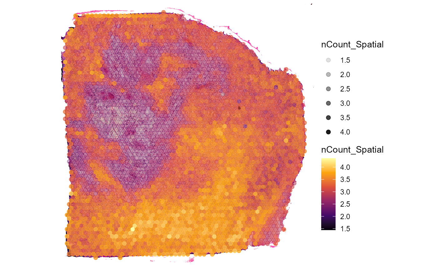

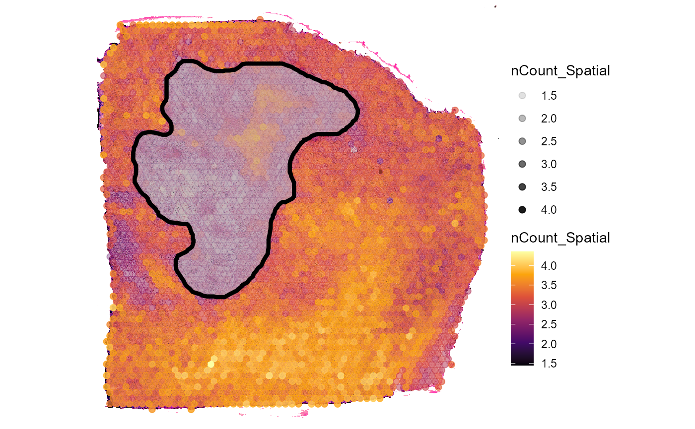
Fig.7 Add the extent of image annotations to surface plots.

5. Working with image annotations

SPATA2 offers several functions that allow to work and program with image annotations. For that we’ll use an example that contains many small image annotations and that is known to contain a highly segregated hypoxic area.

plotImageGgplot(object = object_t275)

plotSurface(
  object = object_t275,
  color_by = "HM_HYPOXIA",
  display_image = FALSE
) + 
  ggpLayerFrameByImage(object_t275)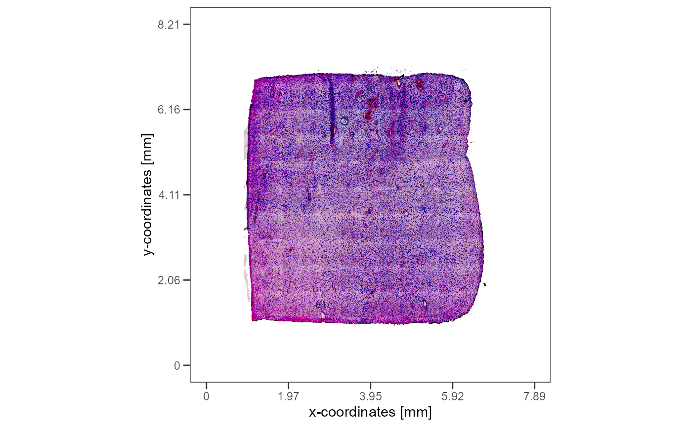

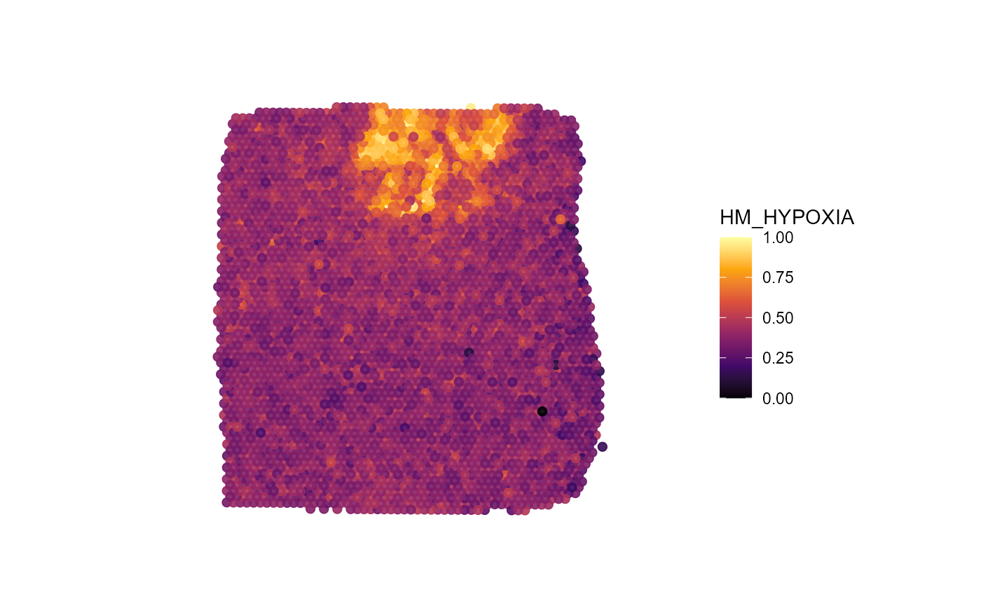
Fig.8 Glioblastoma sample T275 with a prominent hypoxia region.

5.1 Image handling and plotting

We annotated five small vessel that we found in the HE-image using createImageAnnotations() as well as a structure that we assume to be an artifact. Note that the image annotations are provided in the list image_annotations and that these annotations are scaled for the low resolution image.

Arguments expand and square can be used to specify how the cropped image sections are handled. Read the documentation with ?plotImageAnnotations or ?getImageAnnotations for more information.

# load example list 
data("image_annotations")

# set annotations
object_t275 <- 
  setImageAnnotations(
    object = object_t275,
    img_anns = image_annotations[["275_T"]],
    overwrite = TRUE
    )

# plot results (high resolution)
plotImageAnnotations(
  object = object_t275,
  ids = NULL, # no further specification of ids ..
  tags = NULL, # ... and tags includes all image annotations
  expand = 0.4, # expand the image
  square = TRUE, # force the image into a square
  display_subtitle = TRUE, 
  line_size = 1, 
  nrow = 2
  )

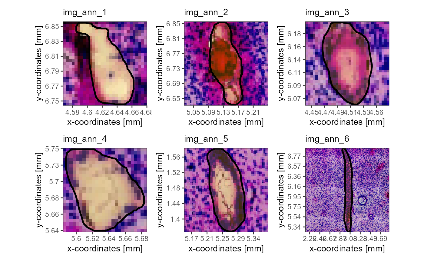
Fig.9 All image annotations of sample T275 one by one in high resolution.

For a visualization of many image annotations on a surface-ggplot you can use ggpLayerImgAnnOutline().

plotImageGgplot(object = object_t275) + 
  ggpLayerImgAnnOutline(
    object = object_t275,
    line_size = 1, 
    line_color = "red"
    )

Fig.10 All image annotations of sample T275 projected on the whole image.

5.2 Using tags

Comparing the localisation of each image annotation from Fig.10 in Fig.11 it becomes apparent that we tagged vessel differently, depending on their position. The tagging system of image annotations can be used to conveniently extract and/or plot image annotations or information thereof. E.g. in Fig.5, the image annotation has been tagged with necrotic and center.

Input for argument tags specifies the tags of interest. Argument test decides about how the specified tags are used to select the image annotations of interest. There are three options:

Argument test set to ‘any’ or 1: To be included, an image annotation must be tagged with at least one of the input tags.
Argument test set to ‘all’ or 2: To be included, an image annotation must be tagged with all of the input tags.
Argument test set to ‘identical’ or 3: To be included, an image annotation must be tagged with all of the input tags and must not be tagged with anything else.
Argument test set to not_identical or 4: To be included, an image annotation must not be tagged with the combination of input tags.
Argument test set to ‘none’ or 5: To be included, an image annotation

Note that the filtering process happens in addition to / after the filtering by input for argument ids. This concept is exemplified in Fig.12 with plotImageAnnotations() but works the same for all other image annotation related functions that extract image annotations.

# plot on the left
plotImageAnnotations(
  object = object_t275, 
  tags = c("vessel", "in_hypoxia"),
  test = "any", # annotations are kept as long as at least one of the tags fit's
  expand = 0.4, 
  square = TRUE
) 

# plot on the right
plotImageAnnotations(
  object = object_t275, 
  tags = c("vessel", "in_hypoxia"),
  test = "all", # to be be kept, all specified tags must be included in the image annoation
  expand = 0.4, 
  square = TRUE, 
  ncol = 3,
  nrow = 2
)

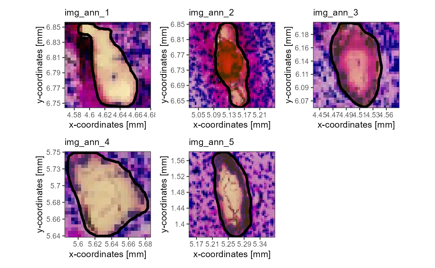
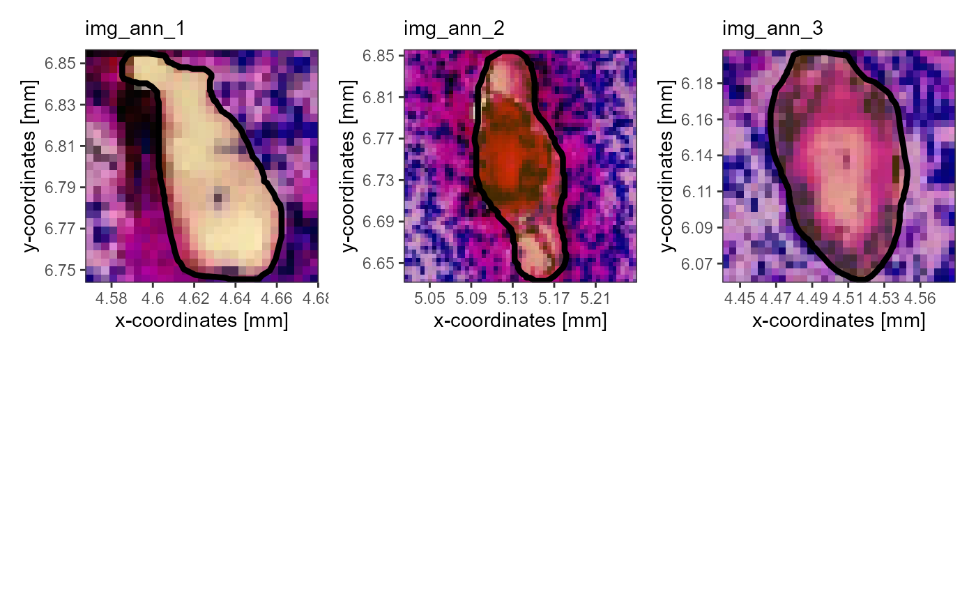
Fig.12 Using tags to specify the image annotations of interest.

Further functions that might be of interest when it comes to integrate histological structures in the analysis or code writing:

# extracts the polygon data.frames that contains the border 
getImgAnnOutlineDf(object = object_t275, tags = "vessel") %>% 
  dplyr::group_by(ids) %>% 
  dplyr::slice_sample(n = 6)

## # A tibble: 30 x 4
## # Groups:   ids [5]
##    ids       border     x     y
##    <fct>     <chr>  <dbl> <dbl>
##  1 img_ann_1 outer  1132. 1659.
##  2 img_ann_1 outer  1123. 1646.
##  3 img_ann_1 outer  1127. 1667.
##  4 img_ann_1 outer  1126. 1644.
##  5 img_ann_1 outer  1136. 1649.
##  6 img_ann_1 outer  1121. 1664.
##  7 img_ann_2 outer  1262. 1628.
##  8 img_ann_2 outer  1248. 1671.
##  9 img_ann_2 outer  1243. 1636.
## 10 img_ann_2 outer  1252. 1671.
## # i 20 more rows

# although image annotations are primarily independent of 
# barcode spots you might want to know which of the barcode spots
# are covered by certain annotations
getImgAnnBarcodes(object = object_t275, tags = "vessel")

## [1] "GAAATACCTGCTGGCT-1" "TGGGCACGTTCTATGG-1" "ATCGGCAAGCAGTCCA-1"
## [4] "CTTCGATTGCGCAAGC-1" "GTGCCTGAGACCAAAC-1"

6. The S4 `ImageAnnotation` class

Image annotations are abstracted in an S4 class named ImageAnnotation. Use ?ImageAnnotation to read the description.

# extracts single image annotations
img_ann <- getImageAnnotation(object = object_t275, id = "img_ann_1")

class(img_ann)

## [1] "ImageAnnotation"
## attr(,"package")
## [1] "SPATA2"

slotNames(img_ann)

## [1] "area"       "id"         "image"      "image_info" "info"      
## [6] "misc"       "tags"

# extracts a list of image annotations
img_anns <- getImageAnnotations(object = object_t275, tags = "vessel", test = "any")

class(img_anns)

## [1] "list"

map(img_anns, .f = class)

## $img_ann_1
## [1] "ImageAnnotation"
## attr(,"package")
## [1] "SPATA2"
## 
## $img_ann_2
## [1] "ImageAnnotation"
## attr(,"package")
## [1] "SPATA2"
## 
## $img_ann_3
## [1] "ImageAnnotation"
## attr(,"package")
## [1] "SPATA2"
## 
## $img_ann_4
## [1] "ImageAnnotation"
## attr(,"package")
## [1] "SPATA2"
## 
## $img_ann_5
## [1] "ImageAnnotation"
## attr(,"package")
## [1] "SPATA2"