Spatial measures - Code & Concept
cc-spatial-measures.Rmd2. Introduction
Many questions researchers try to answer in spatial transcriptomics and image analysis are space related. Coordinates of the observational units - in most cases barcode-spots - are scaled to the resolution of the image that is currently in use. If one exchanges the tissue_lowres_image.png with the tissue_hires_image.png from the 10X Visium output, the coordinates of the barcode-spots are scaled accordingly to ensure that both, coordinates and image, stay aligned. Thus, coordinates can be used to answer spatial questions in relative but not in absolute measures. For instance, the statement: “The necrotic region spans an area of approximately 400pixels.” is useless as the actual area will always depend on the image resolution. The high resolution plot below contains more pixel than the low resolution plot. This affects the coordinate range of the barcode-spots, too, as the ranges of the x- and y-axes display.
library(SPATA2)
library(SPATAData)
library(tidyverse)

# download object
object_t313_highres <- downloadSpataObject(sample_name = "313_T")

# load image annotations
data("image_annotations")

object_t313_highres <-
  setImageAnnotation(
    object = object_t313_highres,
    img_ann = image_annotations[["313_T"]][["necrotic_center"]]
  )

# downscale everything to a low resolution object
object_t313_lowres <- scaleAll(object_t313_highres, scale_fct = 0.25)

# create high and low resolution plots
text_size <- theme(text = element_text(size = 17.5))

low_res_plot <-
  plotImageGgplot(object_t313_lowres, unit = "px") +
  labs(subtitle = "Low resolution") +
  text_size

high_res_plot <-
  plotImageGgplot(object_t313_highres, unit = "px" ) +
  labs(subtitle = "High resolution") +
  text_size

# plot results
low_res_plot

high_res_plot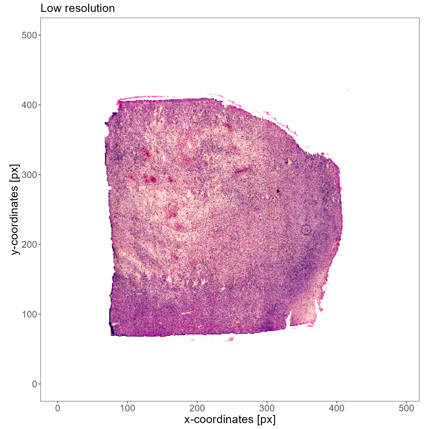
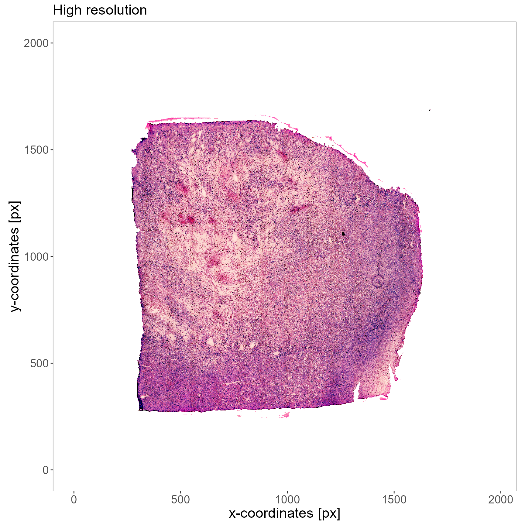
Fig.1 Different resolutions result in different x- and y-scale.
3. The pixel scale factor
To answer questions in absolute measures, distances must be converted to units of the *Système international d’unités (SI). That is, micrometers, millimeters, centimeters, etc. This is possible as most spatial -omic studies come with a ground truth. In case of 10XVisium this ground truth is the center to center distance between two adjacent barcode-spots which is always 100um. Using this information, the actual distances and areas can be computed with a pixel scale factor.
# how many um is one pixel in side lengths
getPixelScaleFactor(object_t313_lowres, unit = "um")
## [1] 17.47339
## attr(,"unit")
## [1] "um/px"
# how many pixel is one um in side lengths
getPixelScaleFactor(object_t313_lowres, unit = "um", switch = TRUE)## [1] 0.05722988
## attr(,"unit")
## [1] "px/um"
# how many um is one pixel in side lengths in case of a higher resolution?
getPixelScaleFactor(object_t313_highres, unit = "um")## [1] 4.368347
## attr(,"unit")
## [1] "um/px"Using scale factors the actual distances can be used in surface plots. Note how the x- and y-axes of the low- and the high resolution plot do not change if they are scaled according to the SI units of length.
# creates axes in SI units
axes_si_low_res <-
ggpLayerAxesSI(
object = object_t313_lowres,
unit = "mm",
breaks_x = str_c(0:8, "mm"), # use mm
breaks_y = str_c(0:8, "mm")
)
axes_si_high_res <-
ggpLayerAxesSI(
object = object_t313_highres, # object that contains the high res. image!
unit = "mm",
breaks_x = str_c(0:8, "mm"),
breaks_y = str_c(0:8, "mm")
)
# plot results
low_res_plot +
axes_si_low_res +
text_size
high_res_plot +
axes_si_high_res +
text_size
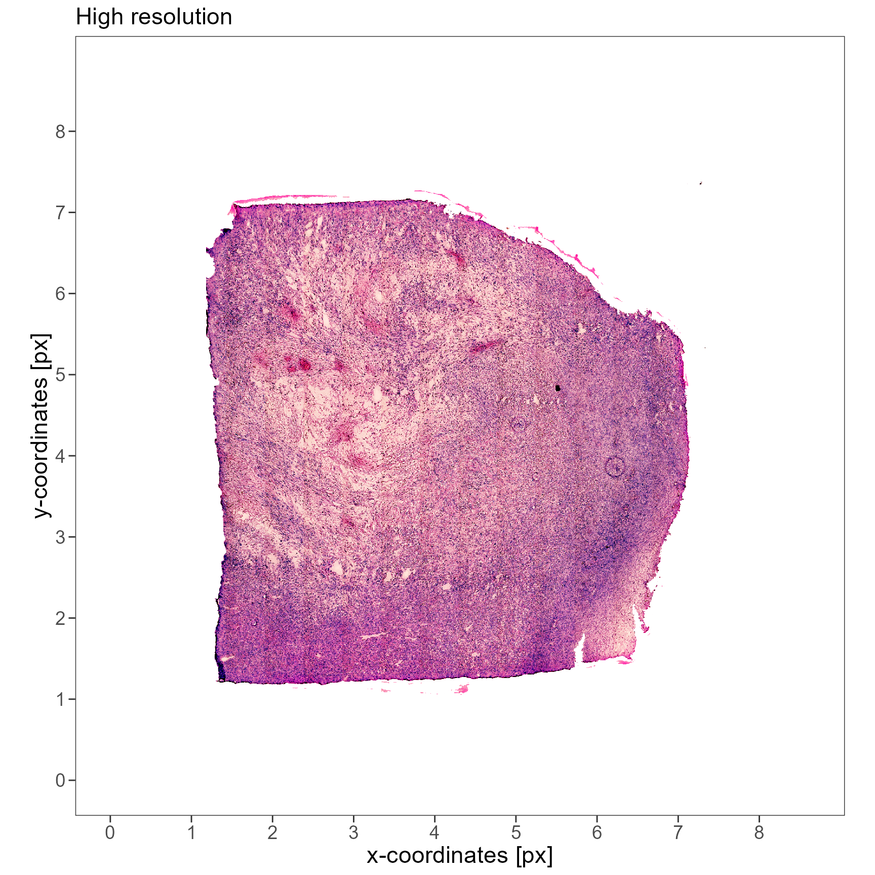
Fig.2 Using SI units results in resolution independent scaling.
The following code chunks show how the pixel scale factor is calculated.
# data.frame with spot to spot distances
bcsp_dist <-
getBarcodeSpotDistances(object_t313_lowres) %>%
dplyr::filter(bc_origin != bc_destination) %>%
dplyr::mutate(dist_round = round(distance, digits = 0))
# keep only spot pairs with the lowest distance to bc_origin
# -> the neighbours
bcsp_dist_neighbors <-
dplyr::group_by(bcsp_dist, bc_origin) %>%
dplyr::filter(dist_round == base::min(dist_round)) %>%
dplyr::mutate(n_neighbors = n()) %>%
dplyr::ungroup() %>%
dplyr::arrange(bc_origin) %>%
dplyr::select(starts_with("bc"), starts_with("distance"), everything())
# if the spot does not lie exactly at the border, a spot has 6 neighbors
bcsp_dist_neighbors## # A tibble: 20,618 x 9
## bc_origin bc_destination distance xo yo xd yd dist_round
## <chr> <chr> <dbl> <dbl> <dbl> <dbl> <dbl> <dbl>
## 1 AAACAAGTATCTCCCA-1 ACTAGTTGCGATC~ 5.71 364. 310. 370. 310. 6
## 2 AAACAAGTATCTCCCA-1 AGAGGCTTCGGAA~ 5.72 364. 310. 361. 315. 6
## 3 AAACAAGTATCTCCCA-1 CAGCAGTCCAGAC~ 5.71 364. 310. 358. 310. 6
## 4 AAACAAGTATCTCCCA-1 GCATCGGCCGTGT~ 5.75 364. 310. 367. 305. 6
## 5 AAACAAGTATCTCCCA-1 GGCAGCAAACCTA~ 5.72 364. 310. 367. 315. 6
## 6 AAACAAGTATCTCCCA-1 TTCTTATCCGCTG~ 5.72 364. 310. 361. 305. 6
## 7 AAACAATCTACTAGCA-1 ATAAACCATTGGA~ 5.71 195. 77.3 201. 77.3 6
## 8 AAACAATCTACTAGCA-1 CGCTACCGCCCTA~ 5.72 195. 77.3 192. 72.4 6
## 9 AAACAATCTACTAGCA-1 CTAAACGGGTGTA~ 5.72 195. 77.3 192. 82.3 6
## 10 AAACAATCTACTAGCA-1 GCGCGATGGGTCA~ 5.71 195. 77.3 198. 72.4 6
## # i 20,608 more rows
## # i 1 more variable: n_neighbors <int>
unique(bcsp_dist_neighbors[["n_neighbors"]])## [1] 6 3 5 4 2 1
# create example df of bcsp with 6 neighbors
six_n <-
dplyr::filter(bcsp_dist_neighbors, n_neighbors == 6) %>%
dplyr::slice_head(n = 6)
six_n## # A tibble: 6 x 9
## bc_origin bc_destination distance xo yo xd yd dist_round
## <chr> <chr> <dbl> <dbl> <dbl> <dbl> <dbl> <dbl>
## 1 AAACAAGTATCTCCCA-1 ACTAGTTGCGATCG~ 5.71 364. 310. 370. 310. 6
## 2 AAACAAGTATCTCCCA-1 AGAGGCTTCGGAAA~ 5.72 364. 310. 361. 315. 6
## 3 AAACAAGTATCTCCCA-1 CAGCAGTCCAGACT~ 5.71 364. 310. 358. 310. 6
## 4 AAACAAGTATCTCCCA-1 GCATCGGCCGTGTA~ 5.75 364. 310. 367. 305. 6
## 5 AAACAAGTATCTCCCA-1 GGCAGCAAACCTAT~ 5.72 364. 310. 367. 315. 6
## 6 AAACAAGTATCTCCCA-1 TTCTTATCCGCTGG~ 5.72 364. 310. 361. 305. 6
## # i 1 more variable: n_neighbors <int>
# create example df of bcsp with 2 neighbors
two_n <-
dplyr::filter(bcsp_dist_neighbors, n_neighbors == 2) %>%
dplyr::slice_head(n = 2)
two_n## # A tibble: 2 x 9
## bc_origin bc_destination distance xo yo xd yd dist_round
## <chr> <chr> <dbl> <dbl> <dbl> <dbl> <dbl> <dbl>
## 1 AGTAGCGTGAACGAAC-1 ACGCCCAGCTGTCG~ 5.72 278. 72.3 275. 77.2 6
## 2 AGTAGCGTGAACGAAC-1 CCTCGACCCACTGC~ 5.72 278. 72.3 281. 77.2 6
## # i 1 more variable: n_neighbors <int>
# use info to color coordinates
levels_loc <- c("Two Neigh.", "Six Neigh.", "Neigh.", "Neither")
plot_df <-
getCoordsDf(object_t313_lowres) %>%
dplyr::mutate(
localisation = dplyr::case_when(
barcodes %in% six_n$bc_origin ~ "Six Neigh.",
barcodes %in% six_n$bc_destination ~ "Neigh.",
barcodes %in% two_n$bc_origin ~ "Two Neigh.",
barcodes %in% two_n$bc_destination ~ "Neigh.",
TRUE ~ "Neither"
),
localisation = factor(x = localisation, levels = levels_loc)
)
plotSurface(
object = plot_df,
color_by = "localisation",
pt_clrp = "Set1",
clrp_adjust = c("Neither" = "lightgrey")
) +
legendColor(size = 10)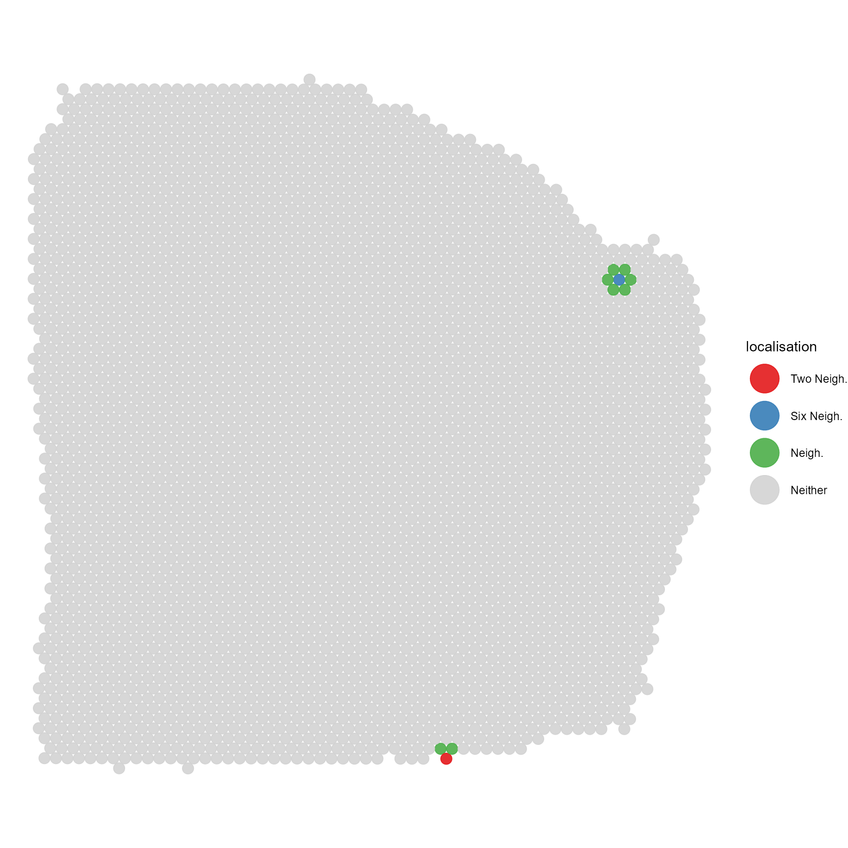
Fig.3 Barcode-spots and their neighbors.
The distance of two neighbors in pixel units can be scaled to the actual distance which is 100um in case of the Visium method.
dist_px <- as.numeric(six_n[1,"distance"])
dist_um <- 100 # 100um
px_scale_fct <- dist_um/dist_px
attr(px_scale_fct, which = "unit") <- "um/px"
px_scale_fct## [1] 17.50901
## attr(,"unit")
## [1] "um/px"
getPixelScaleFactor(object_t313_lowres, unit = "um")## [1] 17.47339
## attr(,"unit")
## [1] "um/px"Note that the distance from one barcode-spot to its neighbors can vary slightly within a few sub pixels. This makes the scale factor vary within the variance of the neighbor to neighbor distance. The algorithm to compute the pixel scale factor takes the median of all neighbor distances to correct for that.
dist_px_corr <- median(bcsp_dist_neighbors[["distance"]])
dist_um <- 100
px_scale_fct_corr <- dist_um/dist_px_corr
attr(px_scale_fct_corr, which = "unit") <- "um/px"
px_scale_fct_corr
## [1] 17.47339
## attr(,"unit")
## [1] "um/px"
getPixelScaleFactor(object_t313_lowres, unit = "um")
## [1] 17.47339
## attr(,"unit")
## [1] "um/px"4. Working with distances
Multiple functions take arguments that, in some way, refer to
distance measures. SPATA2 makes use of the units
package to work with distances. If not explained otherwise in the
documentation you can provide the distance in pixel or in SI units.
Behind the scenes input is converted to pixel and aligned with the
current resolution. 4.1 Converting distances gives some examples of how
this is done.
4.1 Handling distance input and output
Every SI unit of length is a valid distance unit.
validUnitsOfLength()
##  nanometer micrometer millimeter centimeter  decimeter      meter
##       "nm"       "um"       "mm"       "cm"       "dm"        "m"       "px"

validUnitsOfLengthSI()
##  nanometer micrometer millimeter centimeter  decimeter      meter
##       "nm"       "um"       "mm"       "cm"       "dm"        "m"

# wrappers around units::set_units()
as_micrometer(input = "4mm")
## 4000 [um]

as_millimeter(input = "4cm")
## 40 [mm]
Pixel is not a valid distance unit in units. Pixel,
however, are important in image analysis. SPATA2 provides the wrappers
needed to reconcile both. They are named according to the unit of
interest. To transform between pixel and SI units of length the
SPATA2 object must be provided as the scale factor is
needed. See the documentation of ?is_dist to obtain more
information on how distance values must be specified.
### convert from si -> pixel

# example 1: a simple string works
as_pixel(input = "4mm", object = object_t313_lowres)
## [1] 228.9195
## attr(,"unit")
## [1] "px"

# example 2: a unit object works, too
unit_input <- units::set_units(x = 4, value = "mm")

unit_input
## 4 [mm]

class(unit_input)
## [1] "units"

as_pixel(input = unit_input, object = object_t313_highres)
## [1] 915.6781
## attr(,"unit")
## [1] "px"


### convert from pixel -> si

# example 1: simple numeric input is interpreted as pixel
as_millimeter(
  input = c(100, 200, 300),
  object = object_t313_lowres
  )
## Units: [mm]
## [1] 1.747339 3.494678 5.242017
# example 2: strings with px suffix work, too
as_micrometer(
  input = c("50px", "200px", "800px"),
  object = object_t313_highres
)
## Units: [um]
## [1]  218.4174  873.6695 3494.6778
A major advantage of using SI units of length is that the input and
output of functions that depend on space remains the same regardless of
the image resolution that changes with every call to
exchangeImage().
4.2 Examples
The following are a few examples of where actual distances might come into play.
# specifying x- and y-range while handling images
xrange = c("2.5mm", "6.5mm")
yrange = c("0.5mm", "4.5mm")

# where to set the breaks is a measure of distance, too
breaks_x <- str_c(0:8, "mm")
breaks_y <- str_c(0:8, "mm")

rect_add_on <-
  ggpLayerRect(
    object = object_t313_highres,
    xrange = xrange,
    yrange = yrange
    )

plotImageGgplot(
  object = object_t313_highres,
  unit = "mm",
  breaks_x = breaks_x,
  breaks_y = breaks_y
  ) +
  rect_add_on +
  text_size

plotImageGgplot(
  object = object_t313_highres,
  unit = "mm",
  xrange = xrange,
  yrange = yrange,
  breaks_x = breaks_x,
  breaks_y = breaks_y
  ) +
  text_size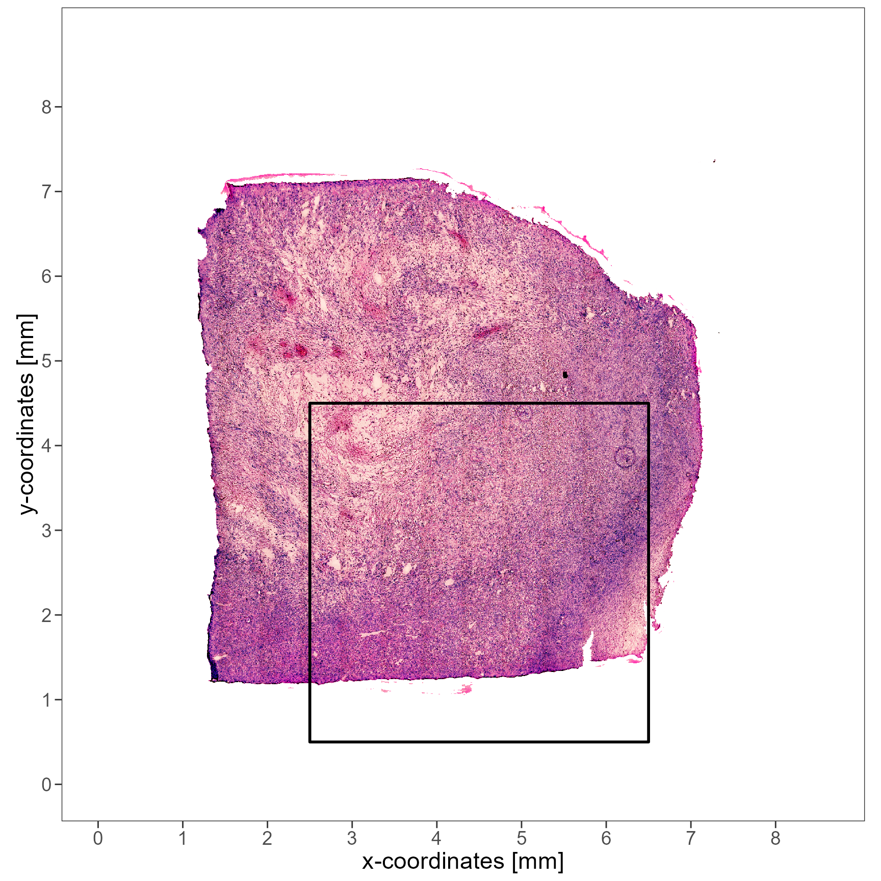
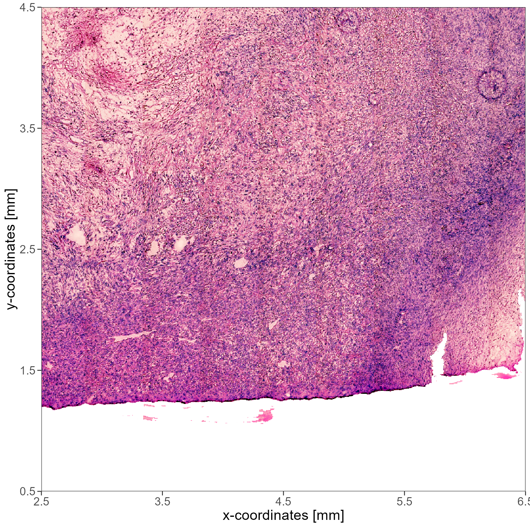
Fig.4 Using SI units to specify distances and ranges.
theme_coords <- ggpLayerThemeCoords()

# low resolution vs high resolution in pixel
# -> different inputs
plotSurfaceIAS(
  object = object_t313_lowres,
  id = "necrotic_center",
  distance = 68.8,
  binwidth = 6.8,
  display_bins_angle = FALSE,
  ggpLayers = list(labs(subtitle = "Low res. - Pixel"), text_size, theme_coords)
)

plotSurfaceIAS(
  object = object_t313_highres,
  id = "necrotic_center",
  distance = 244,
  binwidth = 24.4,
  display_bins_angle = FALSE,
  ggpLayers = list(labs(subtitle = "High res. - Pixel"), text_size, theme_coords)
)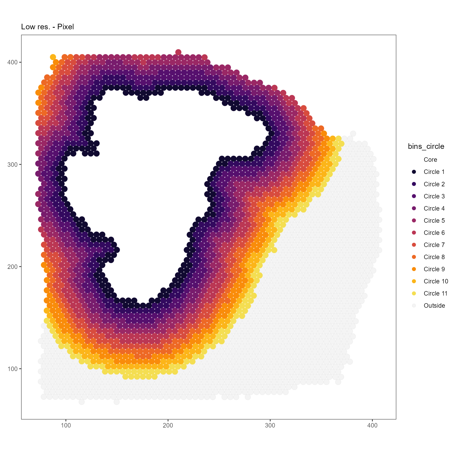
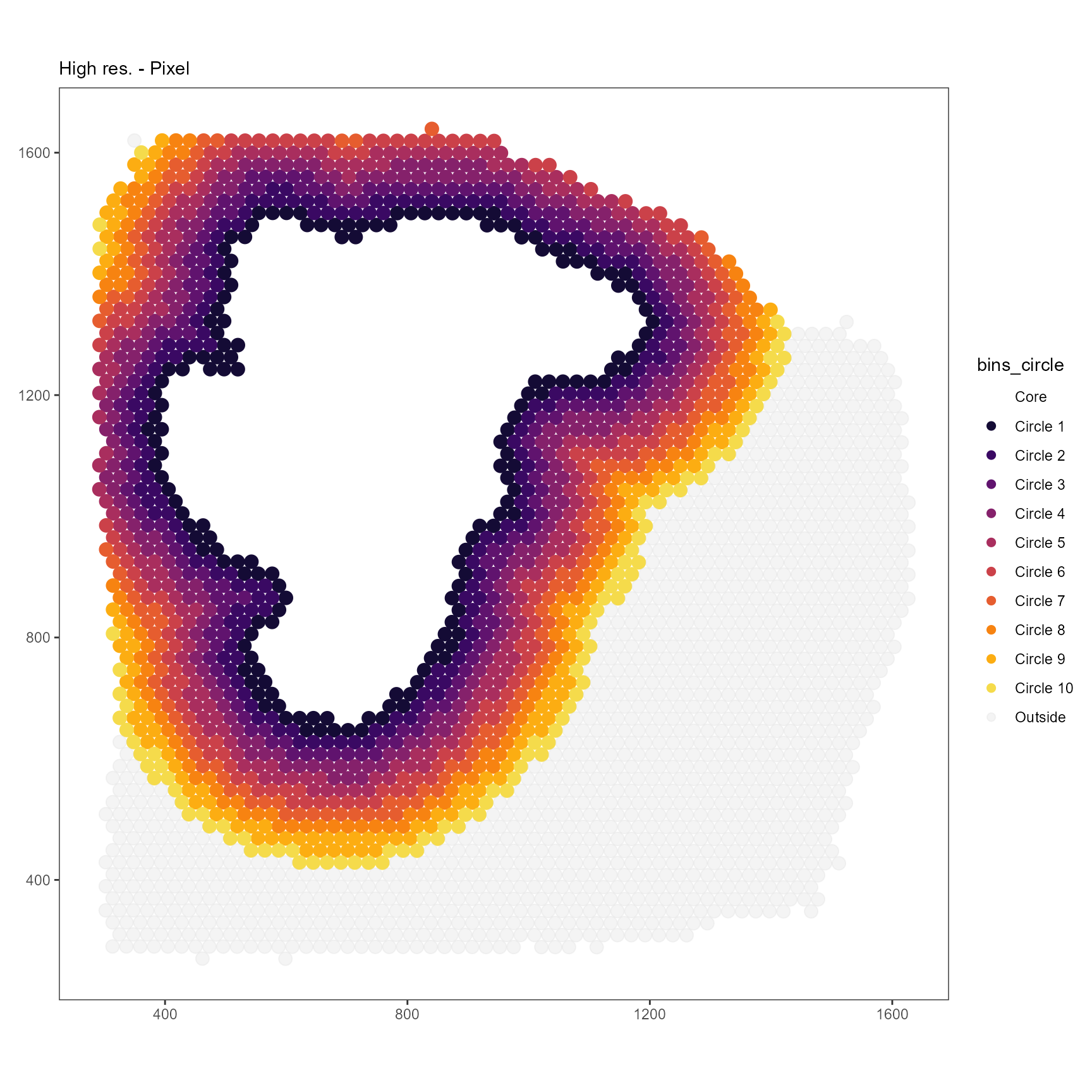
Fig.5 Using pixel lengths is error prone.
The input for distance and binwidth differs
between the two resolution if entered in pixel. One can avoid awkward
and error prone conversions by simply using the same input using SI
units.
# low resolution vs high resolution in si
# -> input remains the same -> output remains the same (regardless of resolution)
plotSurfaceIAS(
  object = object_t313_lowres,
  id = "necrotic_center",
  distance = "2000um",
  binwidth = "200um", # 2000um / 200um = 10
  display_bins_angle = FALSE,
  ggpLayers = list(axes_si_low_res, labs(subtitle = "Low res. - SI"), text_size, theme_coords)
)

plotSurfaceIAS(
  object = object_t313_highres,
  id = "necrotic_center",
  distance = "2000um",
  binwidth = "200um",
  display_bins_angle = FALSE,
  ggpLayers = list(axes_si_high_res, labs(subtitle = "High res. - SI"), text_size, theme_coords)
)
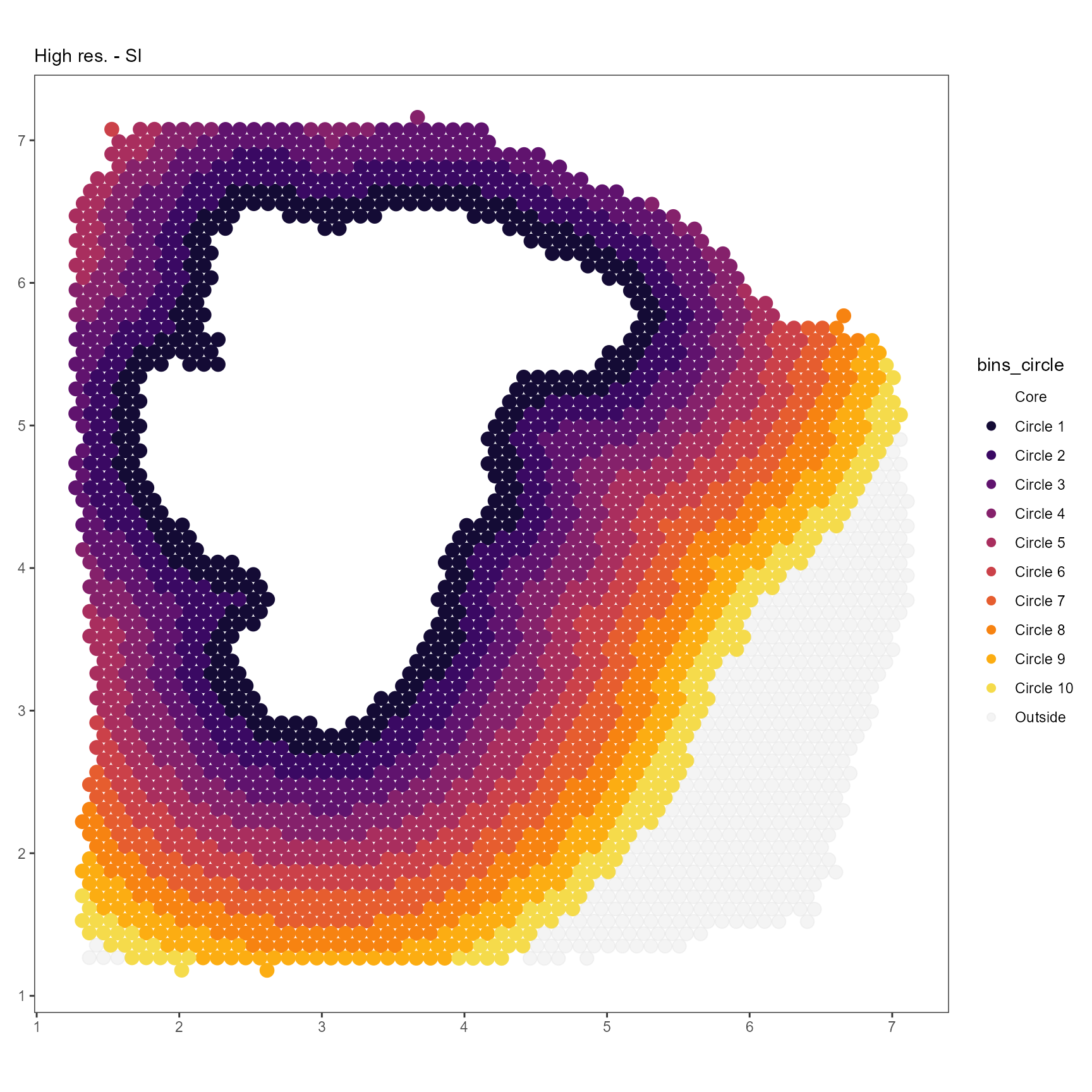
Fig.6 Using SI units to specify algorithm input.
# measuring distances
data("spatial_trajectories")

object_t313_lowres <-
  setTrajectory(
    object = object_t313_lowres,
    trajectory = spatial_trajectories[["313_T"]][["cross"]],
    overwrite = TRUE
    )

trajectory_add_on <-
  ggpLayerTrajectories(
    object = object_t313_lowres,
    ids = "cross",
    size = 1.5
  )

necrotic_add_on <-
  ggpLayerImgAnnOutline(
    object = object_t313_lowres,
    ids = "necrotic_center",
    line_size = 1
  )

plotImageGgplot(
  object = object_t313_lowres,
  unit = "mm",
  frame_by = "coords"
  ) +
  necrotic_add_on +
  trajectory_add_on +
  text_size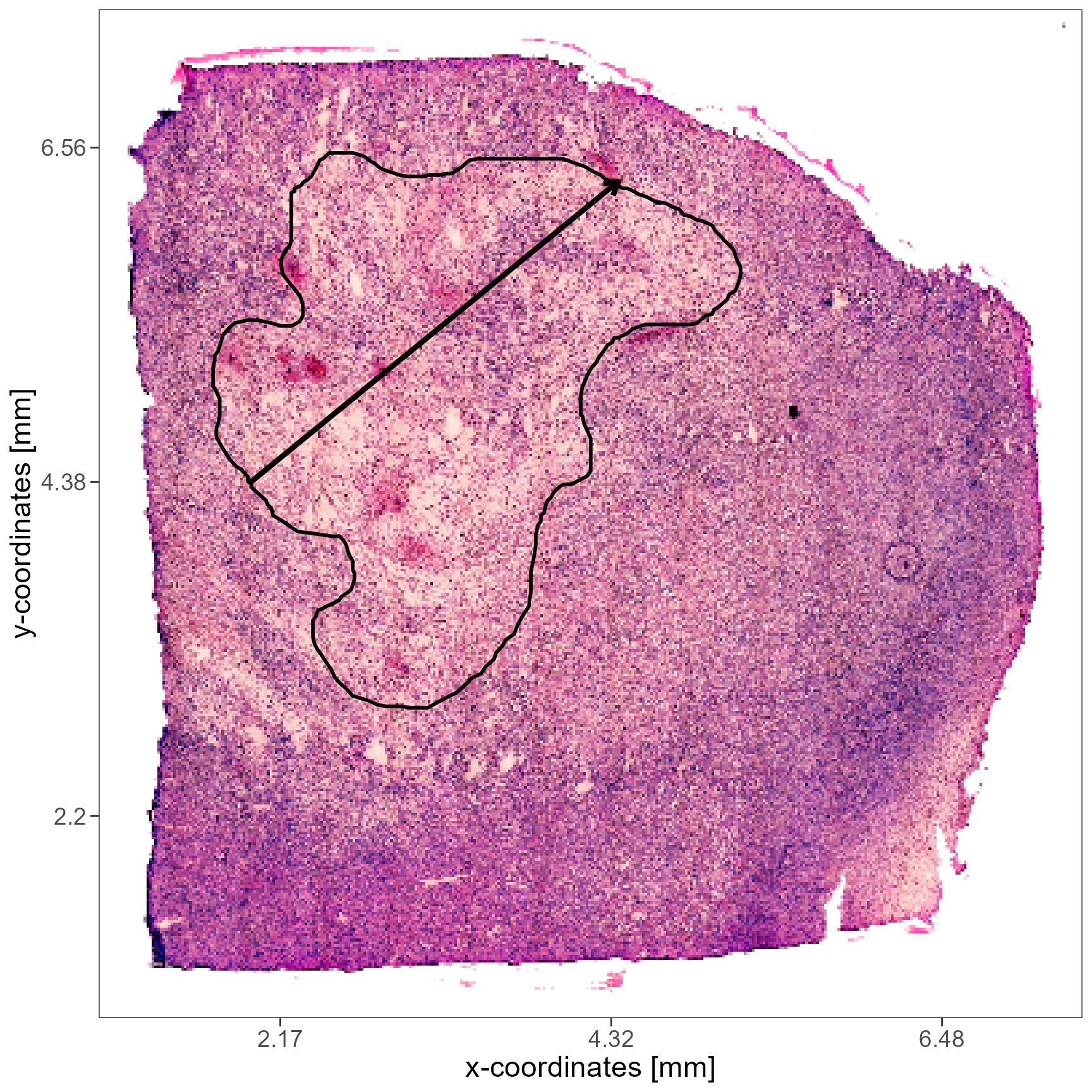
Fig.7 Simplified distance measurement in real space.
# diameter necrotic center
dm_nc <- getTrajectoryLength(object_t313_lowres, id = "cross", unit = "mm")

dm_nc
## 3.106495 [mm]

# always convertable
as_pixel(dm_nc, object = object_t313_lowres)
## [1] 177.7844
## attr(,"unit")
## [1] "px"

as_micrometer(dm_nc)
## 3106.495 [um]
5. Working with areas
In addition to distances, areas can be computed, too. This becomes interesting, for instance, if the area of an image annotation is of relevance to the biological question.
5.1 Handling area input and output
## [1] "nm2" "um2" "mm2" "cm2" "dm2" "m2" "px"Pixel are by definition squares which means that all sides are of the same length. This property is used in SPATA2 to use pixel as a unit of distance. It can, however, be a unit of area, too. E.g. 4px with a side length of 1um cover an area of 4um2 or an area of 4px. However, the number of pixels that cover a specific area again depends on the resolution of the image. Again, SPATA2 implements SI units of area.
## [1] "nm2" "um2" "mm2" "cm2" "dm2" "m2"Pixel is not among them. SPATA2 allows resolution dependent conversion from pixel to SI units and vice versa. As pixel are squares of equal sizes the scale factor used for distance conversion can be used in its squared form.
getPixelScaleFactor(object_t313_lowres, unit = "um2")## [1] 305.3193
## attr(,"unit")
## [1] "um2/px"
# fewer um2 per pixel in the high resolution object
# -> pixels are smaller
getPixelScaleFactor(object_t313_highres, unit = "um2")
## [1] 19.08246
## attr(,"unit")
## [1] "um2/px"Functions that convert areas are named similar to those that convert
distances. If pixels are involved, the SPATA2 object must
be specified as the scale factor is needed.
# numeric input is interpreted as pixel
as_millimeter2(input = c(200, 400, 4000, 50000), object = object_t313_lowres)
## Units: [mm^2]
## [1] 0.06106387 0.12212773 1.22127732 15.26596652
# if character, different units can be specified as input
as_centimeter2(input = c("4mm2", "400px"), object = object_t313_lowres)
## Units: [cm^2]
## [1] 0.040000000 0.0012212775.2 Examples
Compute the area that is covered by the tissue sample.
getSampleAreaSize(object_t313_lowres, unit = "mm2")## 30.69711 [mm^2]Compute the area that is covered by different image annotations and filter accordingly.
# download sample
object_t275_highres <- downloadSpataObject(sample_name = "275_T")

# set image annotations
data("image_annotations")

object_t275_highres <-
  setImageAnnotations(
    object = object_t275_highres,
    img_anns = image_annotations[["275_T"]],
    overwrite = TRUE
  )
Distance and area information can be displayed with scale
bars. Additionally, the argument expand comes in handy
when it comes to extracting or visualizing image sections. Its input is
versatile: There is a whole section in the vignette Image
handling that elaborates on how to use the argument
expand.
plotImageAnnotations(
  object = object_t275_highres,
  tags = c("vessel", "in_hypoxia"),
  test = "all",
  expand = "400um!", # exclam input to fix x- and y-axis to 400um
  square = TRUE,
  dist_sb = "100um", # add distance scale bar
  text_nudge_y = "25um",
  pos = "bottom_right",
  text_color = "white",
  sgmt_color = "white",
  ggpLayers = list(ggpLayerAxesClean())
)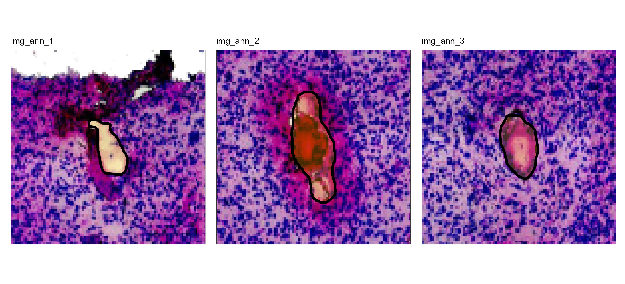
Fig.8 Image annotations whose area can be calculated.
Extracting the values can be used for further subsetting.
img_ann_ids <-
  getImgAnnIds(
    object = object_t275_highres,
    tags = c("vessel", "in_hypoxia"),
    test = "all"
    )

img_ann_areas <-
  getImgAnnArea(
    object = object_t275_highres,
    ids = img_ann_ids,
    unit = "um2"
    )

img_ann_areas
## Units: [um^2]
## img_ann_1 img_ann_2 img_ann_3
## 4951.661 13894.967 7461.176
# subset by annotations of a certain area
threshold <- units::set_units(x = 7500, value = "um2")

img_ann_areas[img_ann_areas > threshold]
## 13894.97 [um^2]