Differential Expression Analysis (DEA) • SPATA2

1. Prerequisites

None.

2. Introduction

Differential expression analysis (DEA) aims to discover quantitative changes in gene expression levels between defined experimental groups. Grouping information is stored in form of grouping variables in the feature data of spata2 object. This includes all spata-intern generated groups such as spatial segmentation and clustering as well as any other grouping variable that has been added via addFeatures().

library(SPATA2)
library(SPATAData)
library(tidyverse)

# download sample 269_T 
object_t269 <- downloadSpataObject(sample_name = "269_T")

object_t269 <- 
  adjustDefaultInstructions(
    object = object_t269, 
    display_image = TRUE,
    clrp = "npg",
    pt_clrp = "npg"
  )

# download sample 275_T 
object_t275 <- downloadSpataObject(sample_name = "275_T")

object_t275 <- 
  adjustDefaultInstructions(
    object = object_t275, 
    display_image = TRUE,
    clrp = "jco",
    pt_clrp = "jco"
  )

# plot histology images 
plotImageGgplot(object = object_t269) + 
  labs(subtitle = "Sample 269_T")

plotImageGgplot(object = object_t275) + 
  labs(subtitle = "Sample 275_T")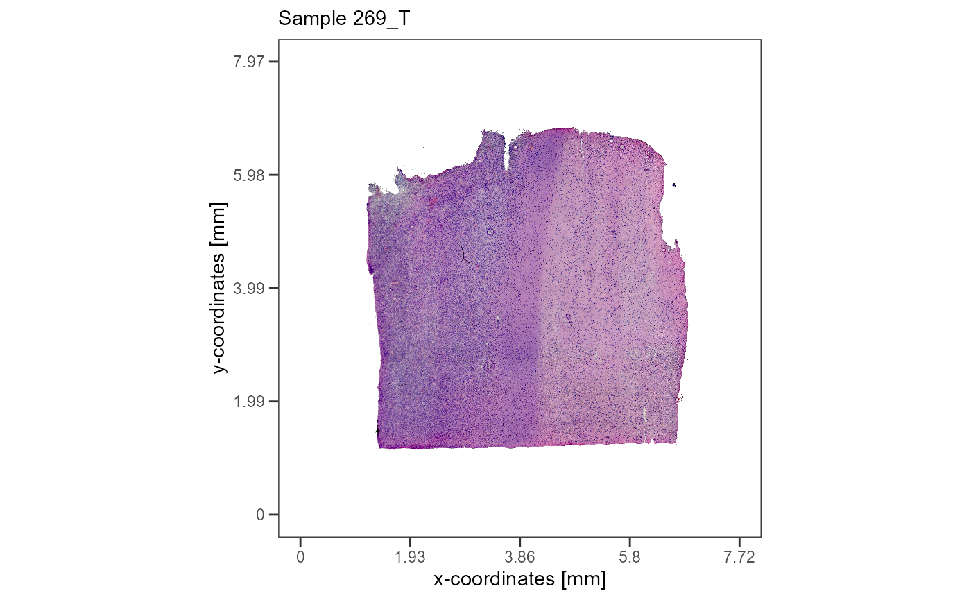

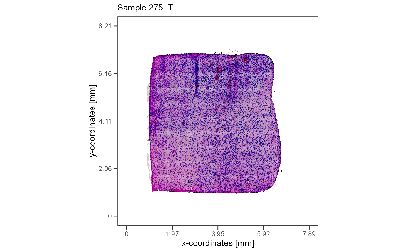
Fig. 1 The histology of the two example samples.

The grouping variables for this tutorial have been prepared before and can be added like the code shows below.

# load histological/spatial segmentation list
data("spatial_segmentations")

# add histology grouping to spata object 
object_t269 <- 
  addFeatures(
    object = object_t269, 
    feature_df = spatial_segmentations[["269_T"]], 
    overwrite = TRUE
  )

getGroupingOptions(object = object_t269)

##            factor            factor 
## "seurat_clusters"       "histology"

# load clustering list
data("snn_clustering")

# add cluster grouping to spata object
object_t275 <- 
  addFeatures(
    object = object_t275, 
    feature_df = snn_clustering[["275_T"]], 
    overwrite = TRUE
  )

getGroupingOptions(object = object_t275)

##            factor            factor            factor 
##     "bayes_space" "seurat_clusters"             "snn"

Visualize the grouping variables with plotSurface().

plotSurface(
  object = object_t269, 
  color_by = "histology"
) 

plotSurface(
  object = object_t275, 
  color_by = "snn"
)

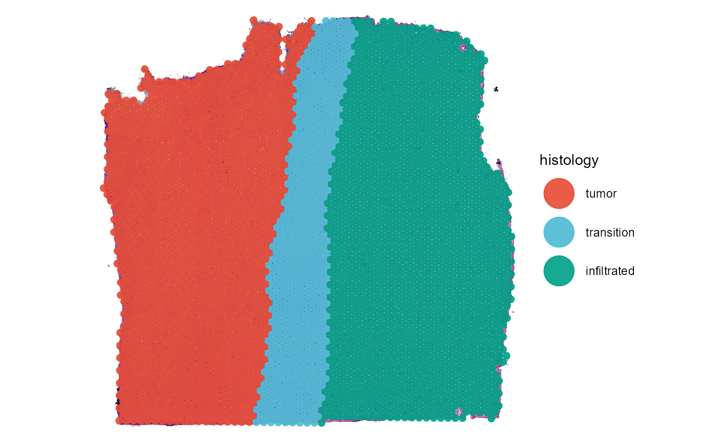
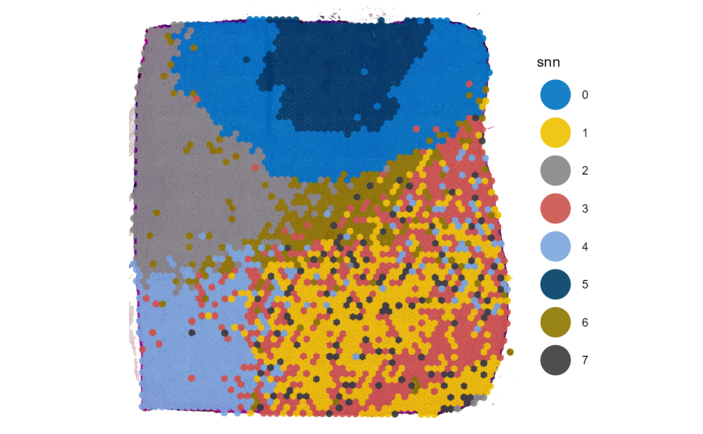
Fig.2 The grouping of the two examples.

3. Running the analysis

DEA in SPATA2 uses the function Seurat::FindAllMarkers(). It’s output is a data.frame in which each row corresponds to a gene that turned out to be a marker gene for one of the identity groups. Additional variables provide information about it’s p-value, adjusted p-value, logFold change etc. runDEA() does not alter the output but stores it in the spata2 object, more precisely in the @dea slot. With printDeaOverview() you can check across which groups and according to which method DEA has already been conducted.

object_t269 <- runDEA(object = object_t269, across = "histology", method_de = "wilcox")

printDeaOverview(object = object_t269)

## DEA results exist for grouping variables:
## 
## - 'seurat_clusters' with methods: wilcox
## - 'histology' with methods: wilcox

object_t275 <- runDEA(object = object_t275, across = "snn", method_de = "wilcox")

printDeaOverview(object = object_t275)

## DEA results exist for grouping variables:
## 
## - 'snn' with methods: wilcox
## - 'bayes_space' with methods: wilcox

3. Extracting results

There are two main functions with which you can manually extract the DEA results desired. First, getDeaResultsDf() returns the original resulting data.frame of Seurat::FindAllMarkers(). getDeaGenes() returns a vector of gene names.

# extract the complete data.frame
getDeaResultsDf(
  object = object_t275, 
  across = "snn", 
  method_de = "wilcox"
)

## # A tibble: 3,786 x 7
##        p_val avg_log2FC pct.1 pct.2 p_val_adj snn   gene  
##        <dbl>      <dbl> <dbl> <dbl>     <dbl> <fct> <chr> 
##  1 7.77e-182      1.27  0.799 0.277 1.67e-177 0     POSTN 
##  2 6.72e-221      1.22  1     0.982 1.44e-216 0     PTN   
##  3 1.89e-233      1.22  1     0.996 4.06e-229 0     CST3  
##  4 4.55e-180      1.18  0.95  0.583 9.75e-176 0     LANCL2
##  5 1.14e-151      0.997 0.925 0.553 2.44e-147 0     TTYH3 
##  6 1.68e-165      0.996 0.995 0.885 3.60e-161 0     HOPX  
##  7 2.08e-158      0.983 0.96  0.699 4.47e-154 0     METRN 
##  8 3.64e-177      0.980 0.995 0.9   7.80e-173 0     RAMP1 
##  9 5.41e-138      0.924 0.994 0.758 1.16e-133 0     RCAN1 
## 10 5.57e-157      0.885 0.997 0.751 1.19e-152 0     IGFBP2
## # i 3,776 more rows

Using the arguments across_subset, min_lfc, n_highest_lfc, max_adj_pval, n_lowest_pval the output of the function can be adjusted to specific questions.

# e.g. top 10 genes for histology area 'tumor' 
getDeaResultsDf(
  object = object_t269, 
  across = "histology",
  across_subset = "tumor", # the group name(s) of interest,
  n_highest_lfc = 10, # top ten genes
  max_adj_pval = 0.01 # pval must be lower or equal than 0.01
)

## # A tibble: 10 x 7
##    p_val avg_log2FC pct.1 pct.2 p_val_adj histology gene    
##    <dbl>      <dbl> <dbl> <dbl>     <dbl> <fct>     <chr>   
##  1     0       2.30 1     0.917         0 tumor     CCT6A   
##  2     0       2.08 1     0.998         0 tumor     SEC61G  
##  3     0       2.03 1     0.879         0 tumor     NIPSNAP2
##  4     0       1.86 0.999 0.909         0 tumor     PTN     
##  5     0       1.82 1     0.834         0 tumor     CD99    
##  6     0       1.79 1     0.977         0 tumor     SPP1    
##  7     0       1.76 1     0.928         0 tumor     PTPRZ1  
##  8     0       1.75 1     0.865         0 tumor     SPARC   
##  9     0       1.72 0.995 0.815         0 tumor     APOC1   
## 10     0       1.60 1     0.844         0 tumor     EGFR

# e.g. all upregulated genes
getDeaResultsDf(
  object = object_t275,
  across = "snn", 
  min_lfc = 0.1 # genes with lfc bigger than or equal to 0.1
)

## # A tibble: 1,953 x 7
##        p_val avg_log2FC pct.1 pct.2 p_val_adj snn   gene  
##        <dbl>      <dbl> <dbl> <dbl>     <dbl> <fct> <chr> 
##  1 7.77e-182      1.27  0.799 0.277 1.67e-177 0     POSTN 
##  2 6.72e-221      1.22  1     0.982 1.44e-216 0     PTN   
##  3 1.89e-233      1.22  1     0.996 4.06e-229 0     CST3  
##  4 4.55e-180      1.18  0.95  0.583 9.75e-176 0     LANCL2
##  5 1.14e-151      0.997 0.925 0.553 2.44e-147 0     TTYH3 
##  6 1.68e-165      0.996 0.995 0.885 3.60e-161 0     HOPX  
##  7 2.08e-158      0.983 0.96  0.699 4.47e-154 0     METRN 
##  8 3.64e-177      0.980 0.995 0.9   7.80e-173 0     RAMP1 
##  9 5.41e-138      0.924 0.994 0.758 1.16e-133 0     RCAN1 
## 10 5.57e-157      0.885 0.997 0.751 1.19e-152 0     IGFBP2
## # i 1,943 more rows

4. Visualize results

4.1 Heatmaps

plotDeaHeatmap() visualizes the results of DEA by using to the results you would extract with getDeaResultsDf().

hm <- 
  plotDeaHeatmap(
    object = object_t275, 
    across = "snn",
    across_subset = c("0", "2", "4", "6"),
    method_de = "wilcox",
    n_highest_lfc = 10, 
    n_bcsp = 100
  )

hm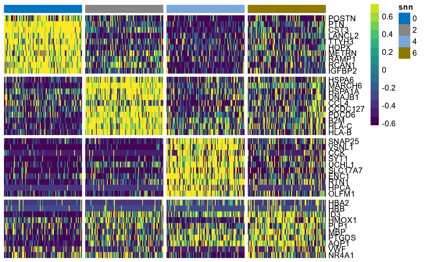

Fig.3 DEA-Heatmap.

4.2 Dotplots

plotDeaDotPlot() visualizes the results of DEA either by group…

plotDeaDotPlot(
  object = object_t275, 
  across = "snn",
  across_subset = c("0", "2", "4"), 
  n_highest_lfc = 5,
  by_group = TRUE, 
  scales = "free_y", 
  ncol = 1
)

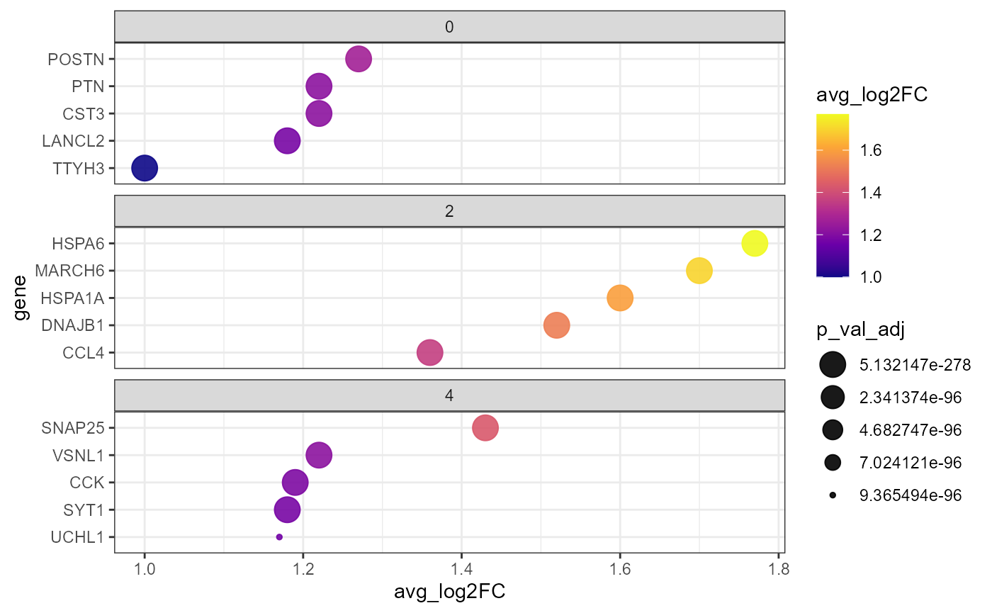
Fig.4 DEA-Dotplot by group.

… or with all groups together.

plotDeaDotPlot(
  object = object_t269, 
  across = "histology",
  color_by = "histology",
  n_highest_lfc = 5, 
  by_group = FALSE
)

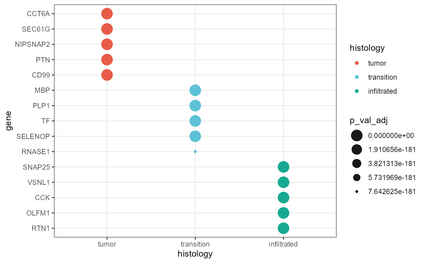
Fig.5 DEA-Dotplot for all groups.

4.3 Box- and Violinplots

There are additional ways to visualize the results of your DEA. As with almost all plotting functions in SPATA2 a vector of gene names is necessary for the function to know which genes to plot. getDeaGenes() is the second function to extract DEA results and a wrapper around getDeaResultsDf() that returns a vector gene names.

genes_of_interest <-
  getDeaGenes(
    object = object_t269,
    across = "histology", # the grouping variable
    method_de = "wilcox", # the method with which the results were computed
    n_highest_lfc = 10, 
    max_adj_pval = 0.01
  )

head(genes_of_interest) # first six

##      tumor      tumor      tumor      tumor      tumor      tumor 
##    "CCT6A"   "SEC61G" "NIPSNAP2"      "PTN"     "CD99"     "SPP1"

tail(genes_of_interest) # last six

## infiltrated infiltrated infiltrated infiltrated infiltrated infiltrated 
##      "RTN1"     "NPAS4"    "SLC1A2"      "BEX1"      "ENC1"      "NRGN"

A vector of gene names as returned by getDeaGenes() is a perfectly valid input for other plotting functions.

top_5_markers_269 <- 
  getDeaGenes(
    object = object_t269,
    across = "histology",
    n_lowest_pval = 5, 
    min_lfc = 0.1 # set min_lfc! else downregulated genes are included
    ) 

top_5_markers_269

##       tumor       tumor       tumor       tumor       tumor  transition 
##     "CCT6A"    "SEC61G"  "NIPSNAP2"       "PTN"      "CD99"      "PLP1" 
##  transition  transition  transition  transition infiltrated infiltrated 
##       "MBP"        "TF"   "SELENOP"       "MAG"    "SNAP25"     "VSNL1" 
## infiltrated infiltrated infiltrated 
##       "CCK"     "OLFM1"      "RTN1"

# plot results for t269
plotBoxplot(
  object = object_t269,
  variables = top_5_markers_269,
  across = "histology", 
  nrow = 3
  ) + 
  theme(axis.text.x = element_blank(), axis.ticks.x = element_blank()) +
  legendTop()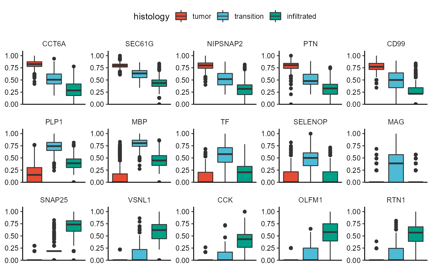

Fig.7 DEA-Boxplots

4.3 Surface plots

Of course, another way to visualize your results are surface plots.

plotSurfaceComparison(
  object = object_t269, 
  color_by = top_5_markers_269 ,
  nrow = 3
  ) + 
  legendNone()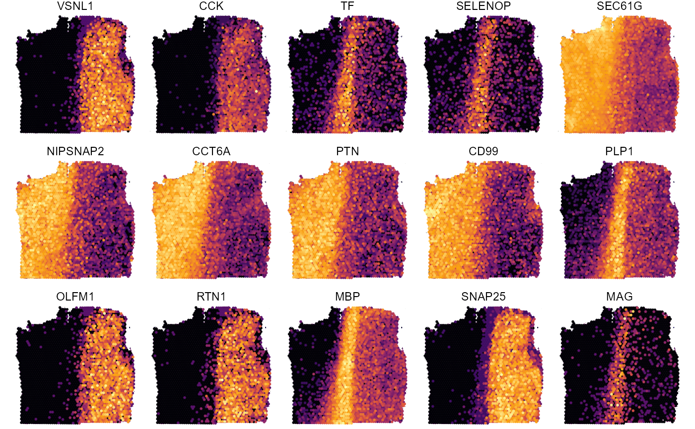

Fig.8 Surface plots with DEA results for sample 269_T.

top_5_markers_275 <- 
  getDeaGenes(
    object = object_t275,
    across = "snn",
    across_subset = c("0", "2", "4"),
    n_lowest_pval = 5, 
    min_lfc = 0.1 # set min_lfc! else downregulated genes are included
    )

plotSurfaceComparison(
  object = object_t275, 
  color_by = top_5_markers_275 ,
  nrow = 3
  ) + 
  legendNone()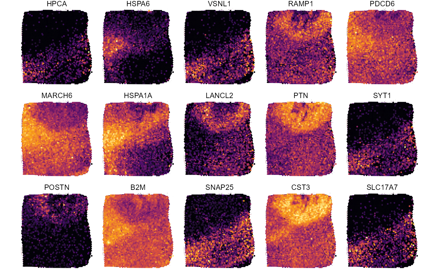

Fig.9 Surface plots with DEA results for sample 275_T.