Gene Set Enrichment Analysis
spata-v2-gsea.Rmd1. Introduction
For a deeper into the results of the DEA one can look for gene sets
that are enriched in the proposed clustering or created based on
histology. SPATA2 implements the hypeR package
which uses hypergeometric testing for enriched gene sets.
# load packages
library(SPATA2)
library(SPATAData)
library(tidyverse)

object_t275 <- downloadSpataObject(sample_name = "275_T")

# load clustering list
object_t275 <-
  setDefault(
    object = object_t275,
    display_image = TRUE,
    clrp = "jco",
    pt_clrp = "jco"
  )

data("snn_clustering")

object_t275 <-
  addFeatures(
    object = object_t275,
    feature_df = snn_clustering[["275_T"]],
    overwrite = TRUE
  )

# histology only
plotSurface(object = object_t275, pt_alpha = 0)

# colored by clustering
plotSurface(object = object_t275, color_by = "snn")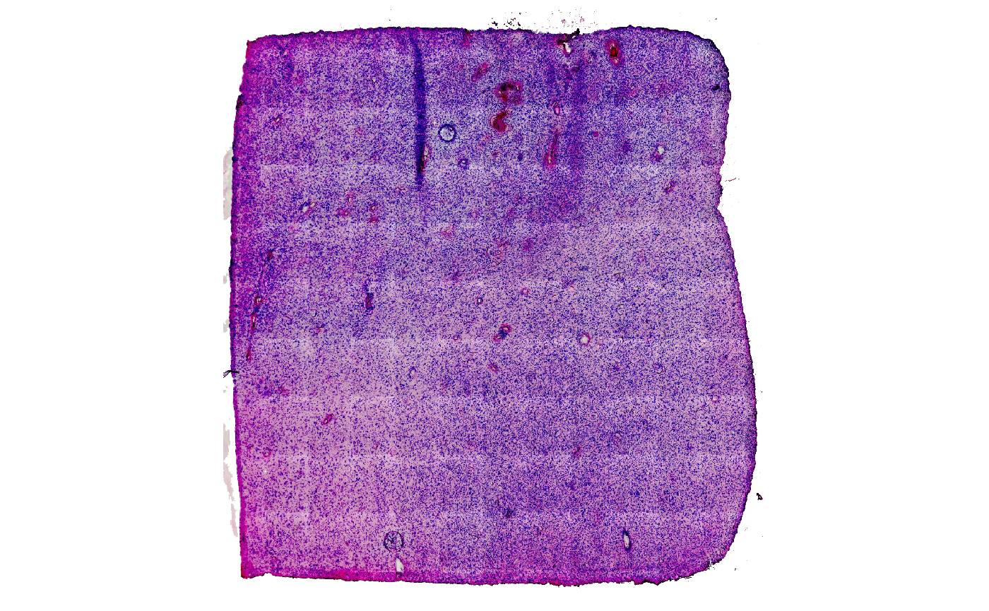
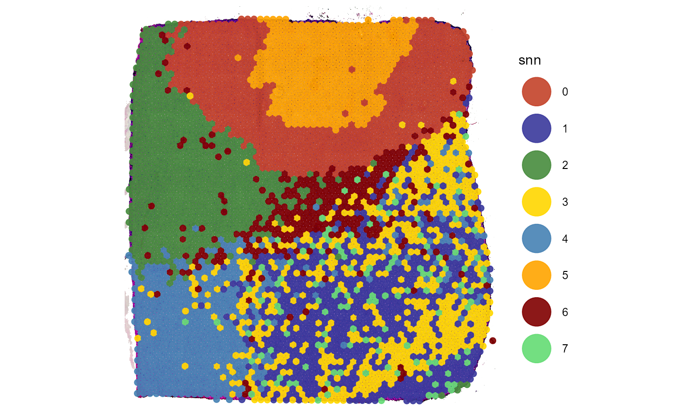
Fig.1 Shared Nearest Neighbour clustering will be analyzed with GSEA.
2. Running the analysis
The function runGSEA() conducts the computation. It
requires the results from runDEA() which conducts the
DE-analysis. By default, the function uses all gene sets that are saved
in the spata2 object. If there are gene sets that you don’t
want to test against you can provide a subsetted list of gene sets.
printGeneSetOverview(object_t275)## Class Available Gene Sets
## 1 BC 289
## 2 BP.GO 7269
## 3 CC.GO 972
## 4 Cell.types 3
## 5 HM 50
## 6 MF.GO 1581
## 7 New 1
## 8 RCTM 1493The default spata2 object contains a variety of gene
sets.
gs_list <- getGeneSetList(object_t275)

length(gs_list)
## [1] 11658For the sake of clarity, his example only uses Biocarta (BC) and Hallmark (HM) gene sets.
# subset gene sets that start with HM or BC
sub_vec <- str_detect(names(gs_list), pattern = "^HM|^BC")

gs_list_sub <- gs_list[sub_vec]

length(gs_list_sub)
## [1] 339Use argument gene_set_list if you want to provide a specific list of
gene sets. Keep it empty if you want to test against all gene sets
stored in the spata2 object.
3. Extracting results
The results can be manually extracted via the following functions.
getGseaResults() extracts a list of hypeR
objects - on for each group. getGseaResultsDf() extracts a
data.frame that results from merging the data of all hypeR
objects together. The group belonging of each gene set is saved in the
variable/column that is named according to the grouping variable - here
snn.
getGseaDf(
  object = object_t275,
  across = "snn",
  method_de = "wilcox",
  n_gsets = 20 # extract top 20 most significant gene sets
)
## # A tibble: 160 x 10
## # Groups: snn [8]
## snn label pval fdr signature geneset overlap background hits
## <fct> <fct> <dbl> <dbl> <int> <int> <int> <int> <chr>
## 1 0 HM_EPITHE~ 3.30e-19 1.10e-16 272 195 26 21441 COL5~
## 2 0 HM_ANGIOG~ 8.3 e- 9 1.4 e- 6 272 34 8 21441 POST~
## 3 0 HM_COMPLE~ 2.20e- 8 2.40e- 6 272 190 15 21441 ADAM~
## 4 0 HM_CHOLES~ 2.8 e- 8 2.40e- 6 272 73 10 21441 ALDO~
## 5 0 HM_COAGUL~ 4.30e- 8 2.90e- 6 272 120 12 21441 TIMP~
## 6 0 HM_GLYCOL~ 1 e- 6 5.10e- 5 272 190 13 21441 PKM,~
## 7 0 HM_APICAL~ 1.10e- 6 5.10e- 5 272 191 13 21441 ITGB~
## 8 0 HM_TNFA_S~ 6 e- 6 2.5 e- 4 272 190 12 21441 F3,J~
## 9 0 HM_UV_RES~ 1.3 e- 5 4.9 e- 4 272 141 10 21441 ANXA~
## 10 0 BC_PLATEL~ 2.3 e- 5 7.8 e- 4 272 14 4 21441 COL4~
## # i 150 more rows
## # i 1 more variable: overlap_perc <dbl>4. Plotting results
Gene set enrichment results can be visualized via dot plots. This can be either done by group with by_group = TRUE or merged for all groups. Figure 2 visualizes the enrichment for cluster 0 and 5 highlighting the hypoxia associated activity in this area.
plotGseaDotPlot(
  object = object_t275,
  across = "snn",
  across_subset = c("0", "5"),
  n_gsets = 10,
  by_group = TRUE,
  transform_with = list(fdr = log10),
  nrow = 2
)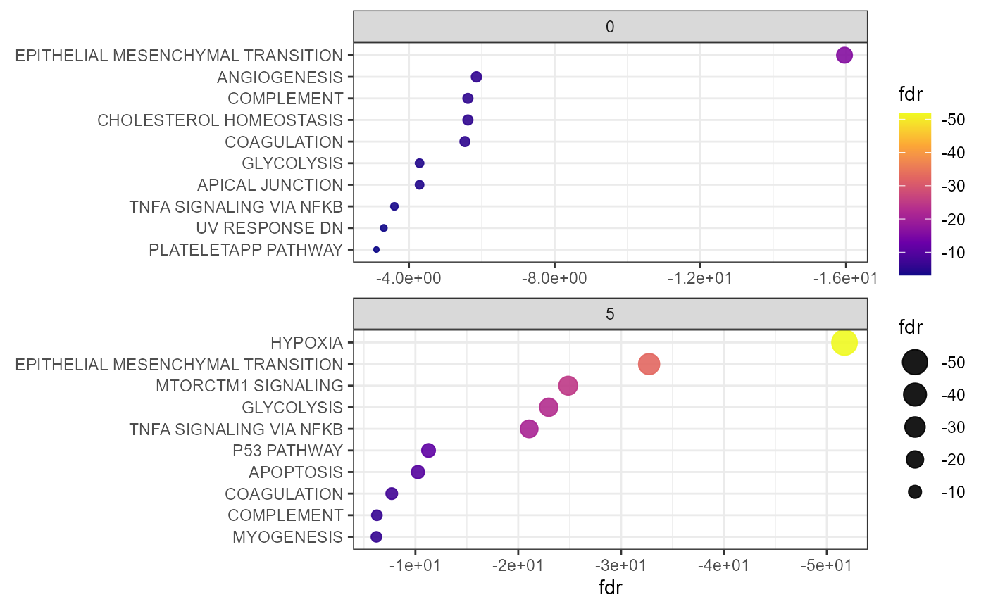
Fig.2 Dot plot to display GSEA results by group.
Using by_group = FALSE the results are merged to one plot. Note that GSEA did not result in any enrichment fo cluster 1 and 3. This might be due to the reduced number of gene sets among which no enriched one was found or due to a low number of upregulated genes.
plotGseaDotPlot(
  object = object_t275,
  across = "snn",
  across_subset = as.character(0:5),
  n_gsets = 7,
  pt_alpha = 0.8,
  transform_with = list(fdr = log10),
  by_group = FALSE # merge in one plot
) 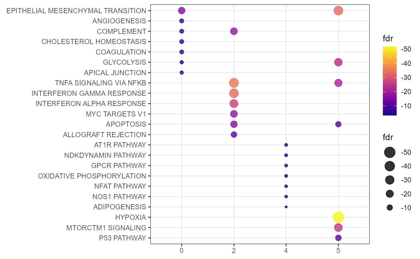
Fig.3 Merged GSEA dot plot.