Spatial Trajectory Screening

1. Prerequisites

Make sure to be familiar with the following vignettes:

2. Introduction & overview

Spatial trajectory screening (STS) fits inferred expression changes of genes to predefined models to screen for genes that follow biologically relevant dynamics along a spatial trajectory. This tutorial gives on overview about the most important functions.

Throughout the tutorial we are using the same example sample that we used in the tutorial on spatial trajectories - the glioblastoma sample T269.

As an example we are using a spatial transcriptomic sample of a central nervous system malignancy that features three different, adjacent histological areas: Tumor, a transition zone as well as infiltrated cortex.

library(SPATA2)
library(SPATAData)
library(tidyverse)

object_t269 <- downloadSpataObject(sample_name = "269_T")

# load example image annotations
data("image_annotations")

object_t269 <- 
  setImageAnnotations(
    object = object_t269, 
    img_anns = image_annotations[["269_T"]],
    overwrite = TRUE
  )

# plot results
plotImageGgplot(object = object_t269) + 
  ggpLayerFrameByCoords(object = object_t269) +
  ggpLayerThemeCoords()

plotImageAnnotations(
  object = object_t269,
  tags = "hist_example", 
  square = TRUE,
  expand = 0.5, 
  encircle = FALSE, 
  nrow = 2, 
  display_caption = FALSE
)

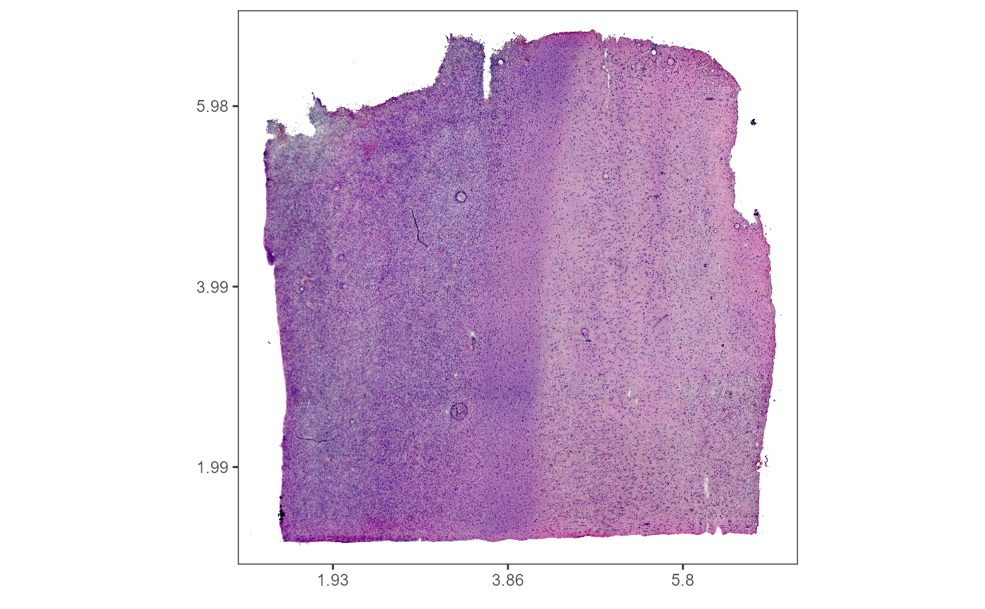
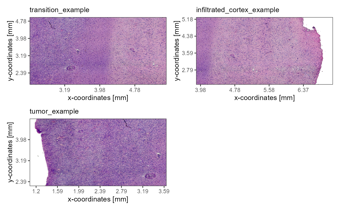
Fig.1 Example sample T269.

The trajectory stays the same, too.

# adds the trajectory that is stored in `spatial_trajectories[["269_T"]][["horizontal_mid"]]`
object_t269 <- 
    addSpatialTrajectory(
    object = object_t269,
    id = "horizontal_mid",
    start = c("1.5mm", "3.5mm") ,
    end = c("6.5mm", "3.5mm") ,
    width = "2mm",
    overwrite = TRUE
  )

plotSpatialTrajectories(
  object = object_t269, 
  ids = "horizontal_mid",
  color_by = "MBP"
)

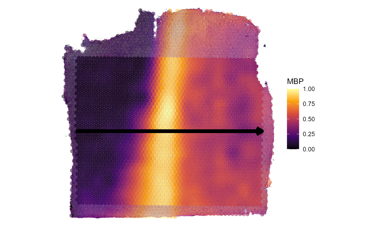
Fig.2 Example spatial trajectory.

3. Run the algorithm

The function to use is called spatialTrajectoryScreening(). The parameter variables takes the numeric variables that are supposed to be included in the screening process. Usually it’s gene names. Spatial trajectory screening, however, is not restricted to genes as virtually every numeric variable (e.g. nCount_Genes, nCount_Features, gene sets, etc.) can be fitted to spatially meaningful models, too. Therefore, the argument for the input is simply called variables.

Here, we are using the genes that were already identified as spatially variable by SPARKX. The goal is to further analyze which of the genes are expressed in a meaningful way along the trajectory.

# this is a wrapper around SPARK::sparkx()
object_t269 <- runSparkx(object = object_t269)

spark_df <- getSparkxGeneDf(object = object_t269, threshold_pval = 0.01)

# extract genes with a sparkx pvalue of 0.01 or lower
sparkx_genes <- spark_df[["genes"]]

# show results
spark_df

# show results (> 10 000 genes detected as spatially variable with a p-value of < 0.01)
str(sparkx_genes)

## # A tibble: 13,839 x 3
##    genes    combinedPval adjustedPval
##    <chr>           <dbl>        <dbl>
##  1 ID3                 0            0
##  2 MARCKSL1            0            0
##  3 PHC2                0            0
##  4 GNG5                0            0
##  5 CNN3                0            0
##  6 RHOC                0            0
##  7 TXNIP               0            0
##  8 S100A10             0            0
##  9 S100A16             0            0
## 10 C1orf61             0            0
## # i 13,829 more rows

##  chr [1:13839] "ID3" "MARCKSL1" "PHC2" "GNG5" "CNN3" "RHOC" "TXNIP" ...

Once you’ve decided on the input you can run the algorithm.

# catchphrases to subset the models that are of interest (use showModels() to check) 
model_subset <- c("sharp_peak", "abrupt_ascending", "abrupt_descending") 

STS_T269 <- 
  spatialTrajectoryScreening(
    object = object_t269, 
    id = "horizontal_mid", # ID of the spatial trajectory
    variables = sparkx_genes, # the variables/genes to scree 
    model_subset = model_subset 
  )

Note: The output of spatialTrajectoryScreening() is not saved in the spata2 object but returned in a separate S4 object of class SpatialTrajectoryScreening. Do not overwrite the spata2 object by writing object_t269 <- spatialTrajectoryScreening(object = object_t269, id = "horizontal_mid", ...).

4. Results

4.1 Visualization

To get an overview of the screening as well as a first visualization of the results use plotOverview(). It sorts genes by their best model-fit and plots the evaluation score against the p-value for every model.

plotOverview(
  object = STS_T269,
  label_vars = 4, # label top 4 variables/genes per model
  label_size = 3
)

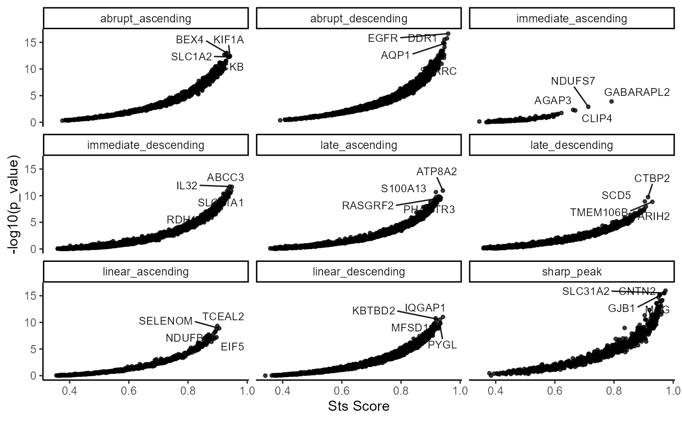
Fig.4 Overview of the screening results.

traj_layer <- 
  ggpLayerTrajectories(
    object = object_t269, 
    ids = "horizontal_mid", 
    size = 2.5
    )

# abrupt descending
plotSurfaceComparison(
  object = object_t269, 
  color_by = c("EGFR", "DDR1")
) + 
  traj_layer + 
  labs(subtitle = "a) Abrupt descending")

# sharp peak
plotSurfaceComparison(
  object = object_t269, 
  color_by = c("CNTN2", "SLC31A2")
) + 
  traj_layer + 
  labs(subtitle = "b) Sharp peak")

# abrupt ascending
plotSurfaceComparison(
  object = object_t269, 
  color_by = c("BEX4", "KIF1A")
) + 
  traj_layer + 
  labs(subtitle = "c) Abrupt ascending")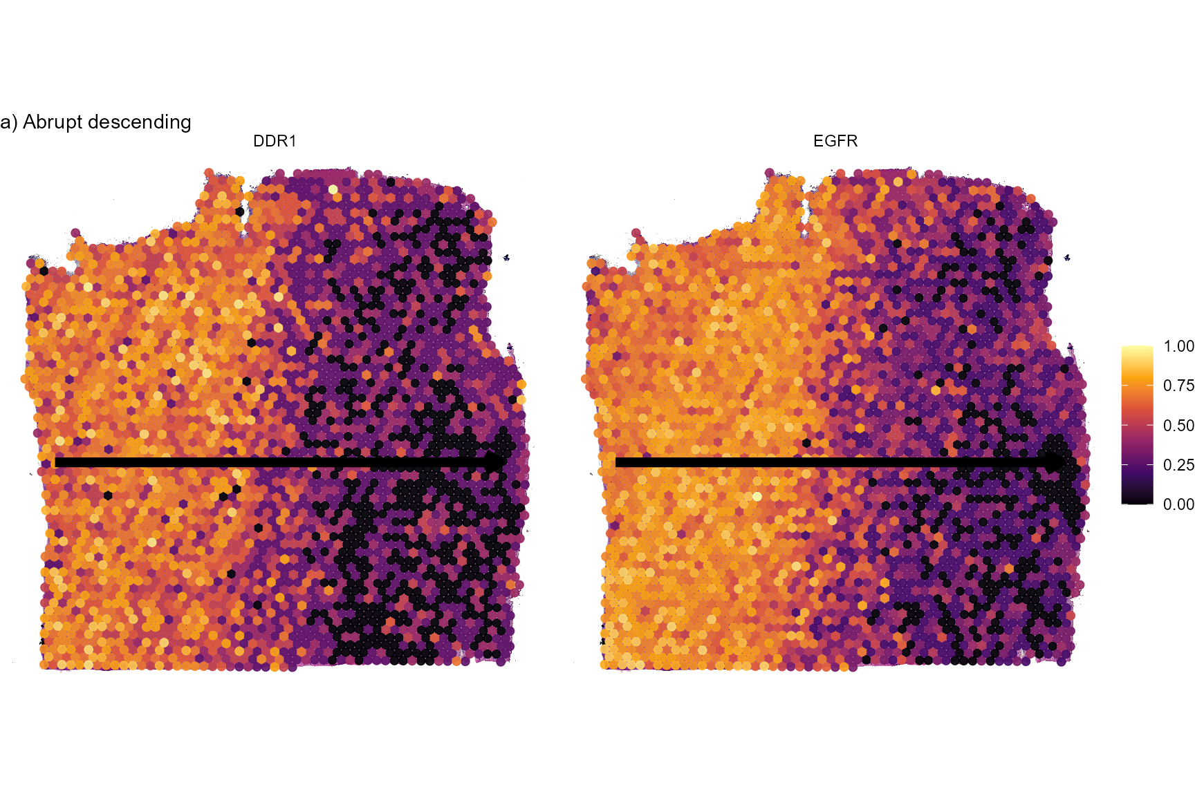

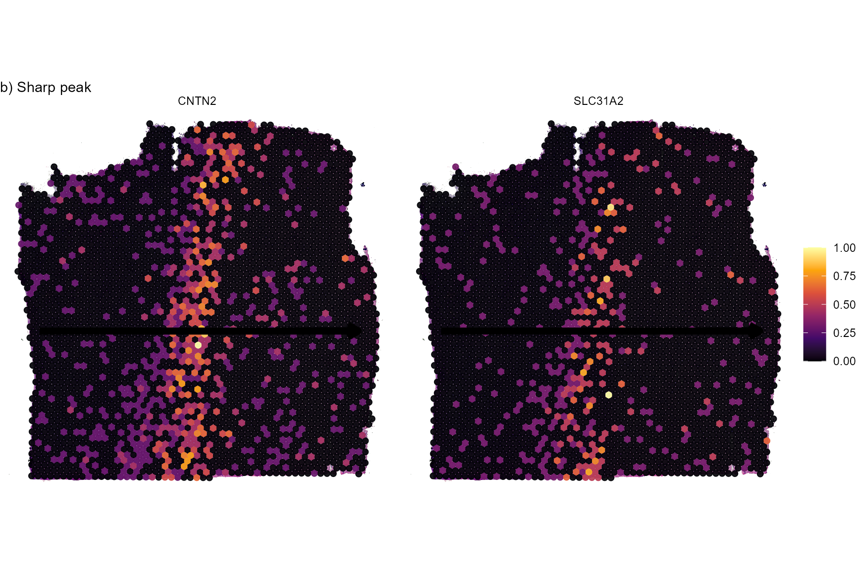
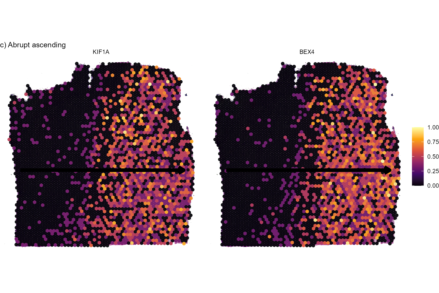
Fig.5 Surface plots of screening results.

Fig.5 Surface plots of screening results.

The inferred gene expression can be visualized with plotTrajectoryLineplot().

plotTrajectoryLineplot(
  object = object_t269, 
  id = "horizontal_mid", 
  variables = c("EGFR", "DDR1", "CNTN2", "SLC31A2", "BEX4", "KIF1A"), 
  clrp = "sifre",
  nrow = 2
)

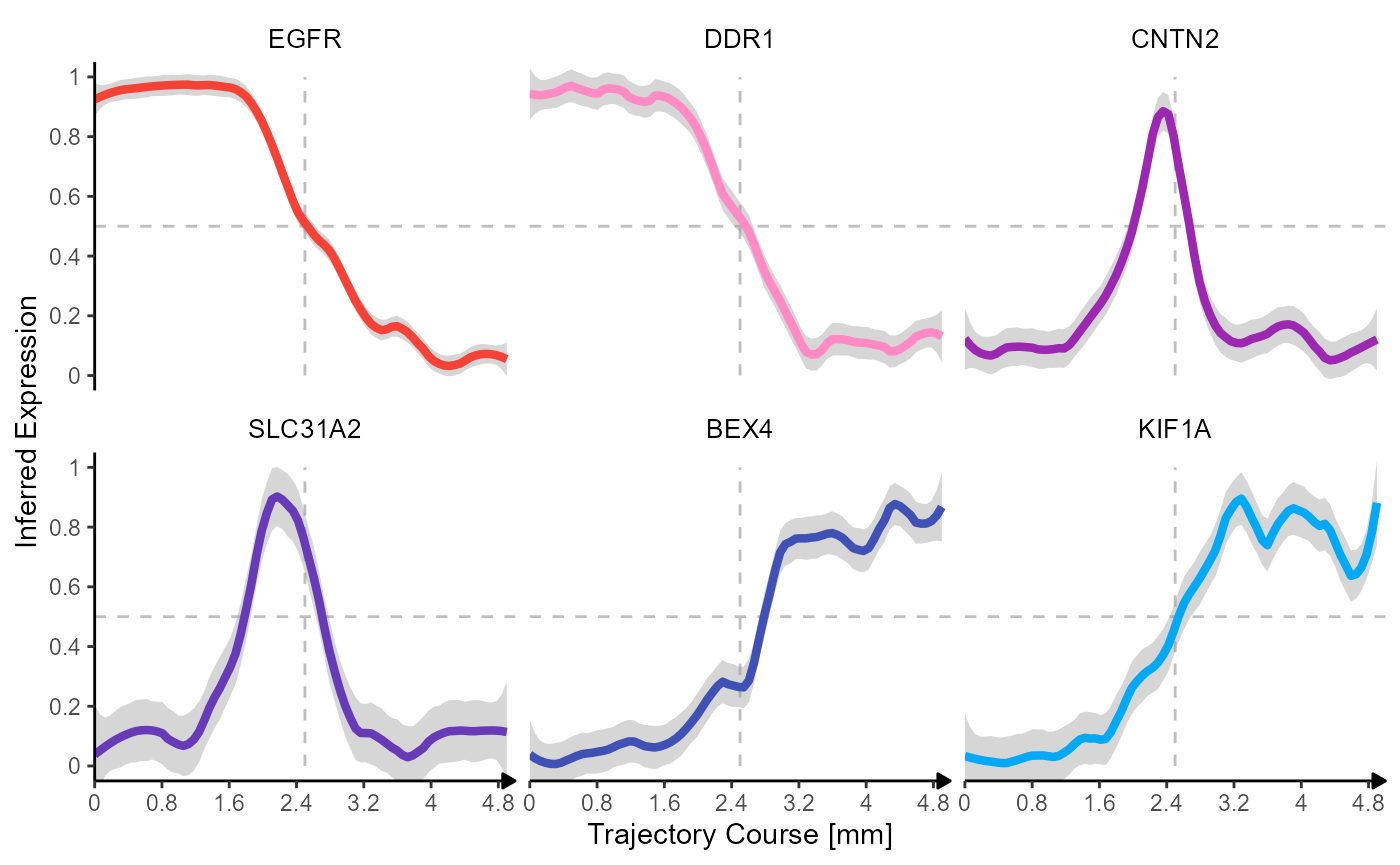
Fig.6 Trajectory lineplots of inferred expression changes.

The used models can always be visualized with showModels().

showModels(model_subset = model_subset)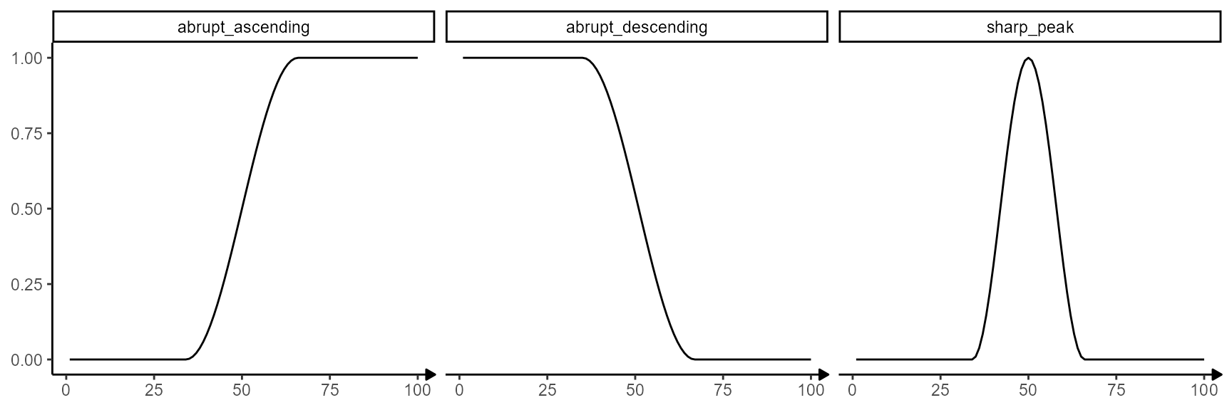

Fig.7 The models that were screened for.

4.2 Extract results

Results can be extracted as data.frames with getResultsDf() or as a character vector of variable/gene names with getResultsVec().

res_df <- 
  getResultsDf(object = STS_T269) %>% 
  head(200)

res_df

## # A tibble: 200 x 8
## # Groups:   models [1]
##    variables models        sts_score  corr  raoc  p_value  rauc p_value_adjusted
##    <chr>     <chr>             <dbl> <dbl> <dbl>    <dbl> <dbl>            <dbl>
##  1 KIF1A     abrupt_ascen~     0.942 0.970 0.914 3.73e-13  1.81         3.44e-10
##  2 SLC1A2    abrupt_ascen~     0.940 0.969 0.912 5.28e-13  1.85         4.39e-10
##  3 CKB       abrupt_ascen~     0.936 0.969 0.903 5.83e-13  2.04         4.66e-10
##  4 BEX4      abrupt_ascen~     0.931 0.974 0.887 9.47e-14  2.37         1.27e-10
##  5 ATP1B1    abrupt_ascen~     0.929 0.962 0.895 3.27e-12  2.21         1.63e- 9
##  6 RTN4      abrupt_ascen~     0.928 0.973 0.883 1.61e-13  2.45         1.89e-10
##  7 BEX2      abrupt_ascen~     0.928 0.963 0.893 2.90e-12  2.25         1.52e- 9
##  8 SLC17A7   abrupt_ascen~     0.927 0.959 0.896 7.33e-12  2.19         2.83e- 9
##  9 RAB11FIP4 abrupt_ascen~     0.924 0.948 0.900 7.31e-11  2.10         1.56e- 8
## 10 CALM2     abrupt_ascen~     0.924 0.956 0.891 1.41e-11  2.29         4.54e- 9
## # i 190 more rows

# top 3 peaking genes
peaking_genes <- 
  getResultsVec(
    object = STS_T269, 
    threshold_eval = 0.5,
    threshold_pval = 0.05,
    model_subset = "sharp_peak"
  ) %>% 
  head(3)

plotSurfaceComparison(
  object = object_t269, 
  color_by = peaking_genes
)

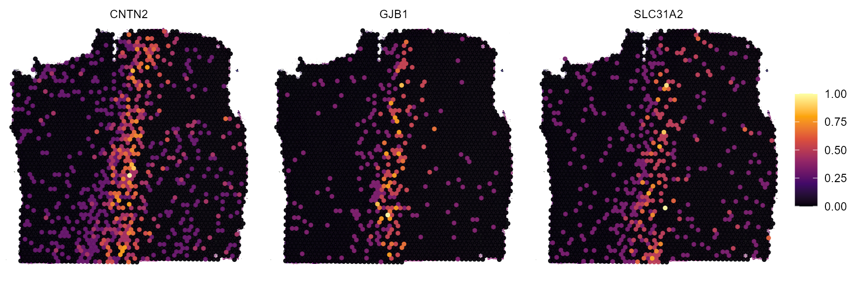
Fig.8 Surface plots of screening results.

5. The S4 `SpatialTrajectoryScreening` class

Spatial trajectory screening results are provided in an S4 object of class SpatialTrajectoryScreening. Use ?SpatialTrajectoryScreening to read the description. Note that SpatialTrajectoryScreening is the class name. spatialTrajectoryScreening() is the function that runs the algorithm.

class(STS_T269)

## [1] "SpatialTrajectoryScreening"
## attr(,"package")
## [1] "SPATA2"

slotNames(STS_T269)

##  [1] "binwidth"           "coords"             "id"                
##  [4] "method_padj"        "models"             "n_bins"            
##  [7] "results"            "sample"             "summarize_with"    
## [10] "spatial_trajectory"