Single Cell Deconvolution
spata-v2-scd.Rmd1. Introduction
Multiple algorithms for single cell deconvolution have been published
that allow to map single cell sequencing data sets in the spatial
dimensions of a Visium data set generated from the same tissue.
SPATA2 offers functions to visualize that and to integrate
the positioning of cells in gradient screening. The data set used is an
injured mouse cortex slice as has been published by Koupourtidou
et al. 2023.
The injuries have been integrated in our analysis using the image annotations system. They were called inj1 and inj2.
library(SPATA2)
library(tidyverse)

# load data set
object_mci <- downloadloadPubExample("MCI_LMU")

# set default and image annotations
object_mci <- setDefault(object_mci, clrp = "sifre", pt_clrp = "sifre")

data("image_annotations")

object_mci <-
  setImageAnnotations(
    object = object_mci,
    img_anns = image_annotations[["MCI_LMU"]],
    overwrite = TRUE
    )

injury_add_on <-
  ggpLayerImgAnnOutline(object_mci, ids = c("inj1", "inj2"))

# get single cell data set
data("sc_deconvolution")
sc_mci <- sc_deconvolution[["MCI_LMU"]]

# plot example data
plotSurface(object_mci, color_by = "clusters") +
  injury_add_on

plotSurface(sc_mci, color_by = "cell_type", pt_clrp = "sifre", pt_size = 1.5) +
  injury_add_on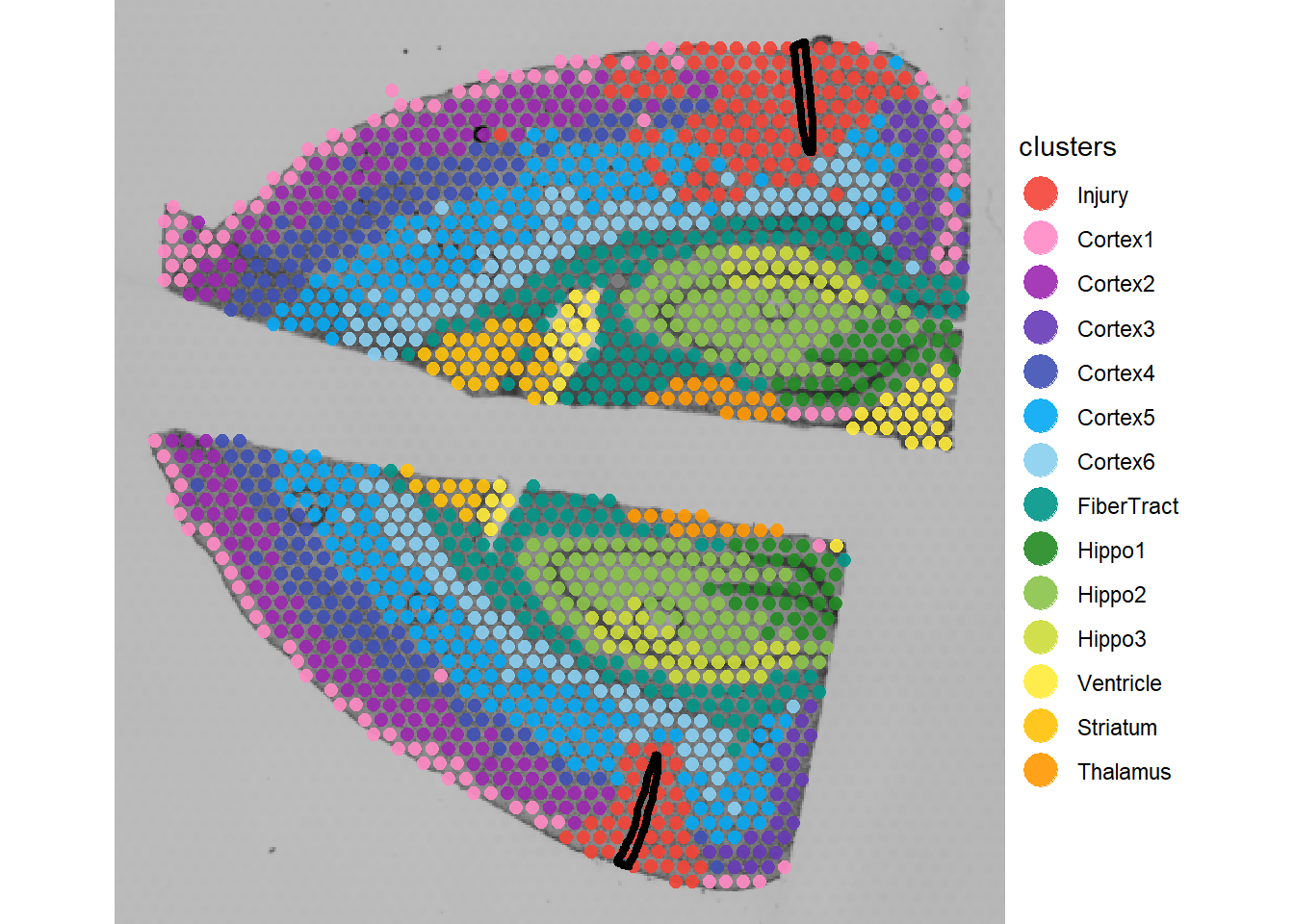
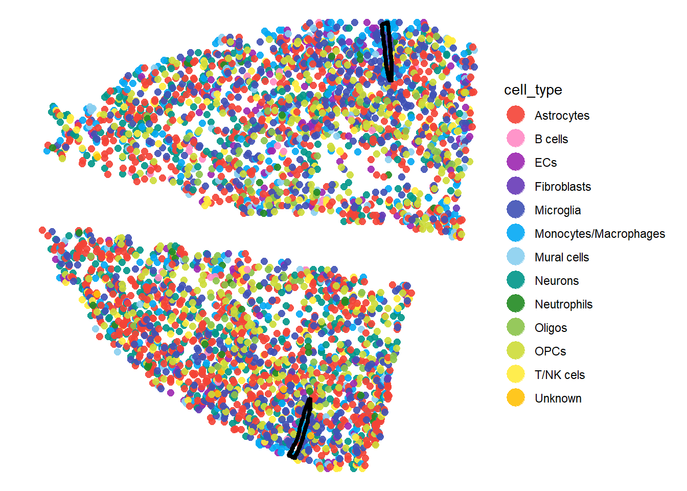
Fig.1 The injured mouse cortex sample clustered and with deconvolution single cell data.
2. Single Cell input
Most function that integrate single cell deconvolution take the
single cell input via the argument sc_input. It expects a
data.frame that contains at least the columns x and y
as numeric pixel coordinates and a factor column called
cell_type.
sc_mci## # A tibble: 4,356 x 7
## x y cell_type spot_id barcodes x_mm y_mm
## <dbl> <dbl> <fct> <chr> <chr> [mm] [mm]
## 1 442. 378. Neurons AAACAAGTATCTCCCA-1_0 AAACAAGTA~ 5.83 4.98
## 2 412. 140. Mural cells AAACAGAGCGACTCCT-1_0 AAACAGAGC~ 5.42 1.85
## 3 412. 137. Astrocytes AAACAGAGCGACTCCT-1_1 AAACAGAGC~ 5.43 1.81
## 4 413. 142. Astrocytes AAACAGAGCGACTCCT-1_2 AAACAGAGC~ 5.44 1.87
## 5 412. 138. Microglia AAACAGAGCGACTCCT-1_3 AAACAGAGC~ 5.43 1.82
## 6 424. 447. Monocytes/Macrophages AAACATTTCCCGGATT-1_0 AAACATTTC~ 5.58 5.89
## 7 425. 452. Microglia AAACATTTCCCGGATT-1_1 AAACATTTC~ 5.60 5.96
## 8 426. 450. Microglia AAACATTTCCCGGATT-1_2 AAACATTTC~ 5.62 5.93
## 9 492. 341. OPCs AAACCCGAACGAAATC-1_0 AAACCCGAA~ 6.48 4.50
## 10 494. 346. OPCs AAACCCGAACGAAATC-1_1 AAACCCGAA~ 6.51 4.56
## # i 4,346 more rowsFurther columns are optional. For this vignette the three mentioned above suffice.
cell_types <- c("Astrocytes", "Monocytes/Macrophages", "Neurons", "Microglia")

sc_mci <-
  filter(sc_mci, cell_type %in% {{cell_types}}) %>%
  mutate(cell_type = droplevels(cell_type)) %>%
  select(x, y, cell_type)

sc_mci
## # A tibble: 3,221 x 3
## x y cell_type
## <dbl> <dbl> <fct>
## 1 442. 378. Neurons
## 2 412. 137. Astrocytes
## 3 413. 142. Astrocytes
## 4 412. 138. Microglia
## 5 424. 447. Monocytes/Macrophages
## 6 425. 452. Microglia
## 7 426. 450. Microglia
## 8 215. 391. Monocytes/Macrophages
## 9 215. 390. Astrocytes
## 10 215. 393. Astrocytes
## # i 3,211 more rows3. Visualization
To visualize the cells in space use plotSurfaceSC().
injury_add_on_thin <-
  ggpLayerImgAnnOutline(object_mci, ids = c("inj1", "inj2"), line_size = 0.5)

plotSurfaceSC(
  object = object_mci,
  sc_input = sc_mci,
  cell_types = cell_types,
  display_image = TRUE,
  display_density = FALSE,
  display_facets = TRUE,
  pt_size = 0.5,
) +
  injury_add_on_thin +
  legendNone()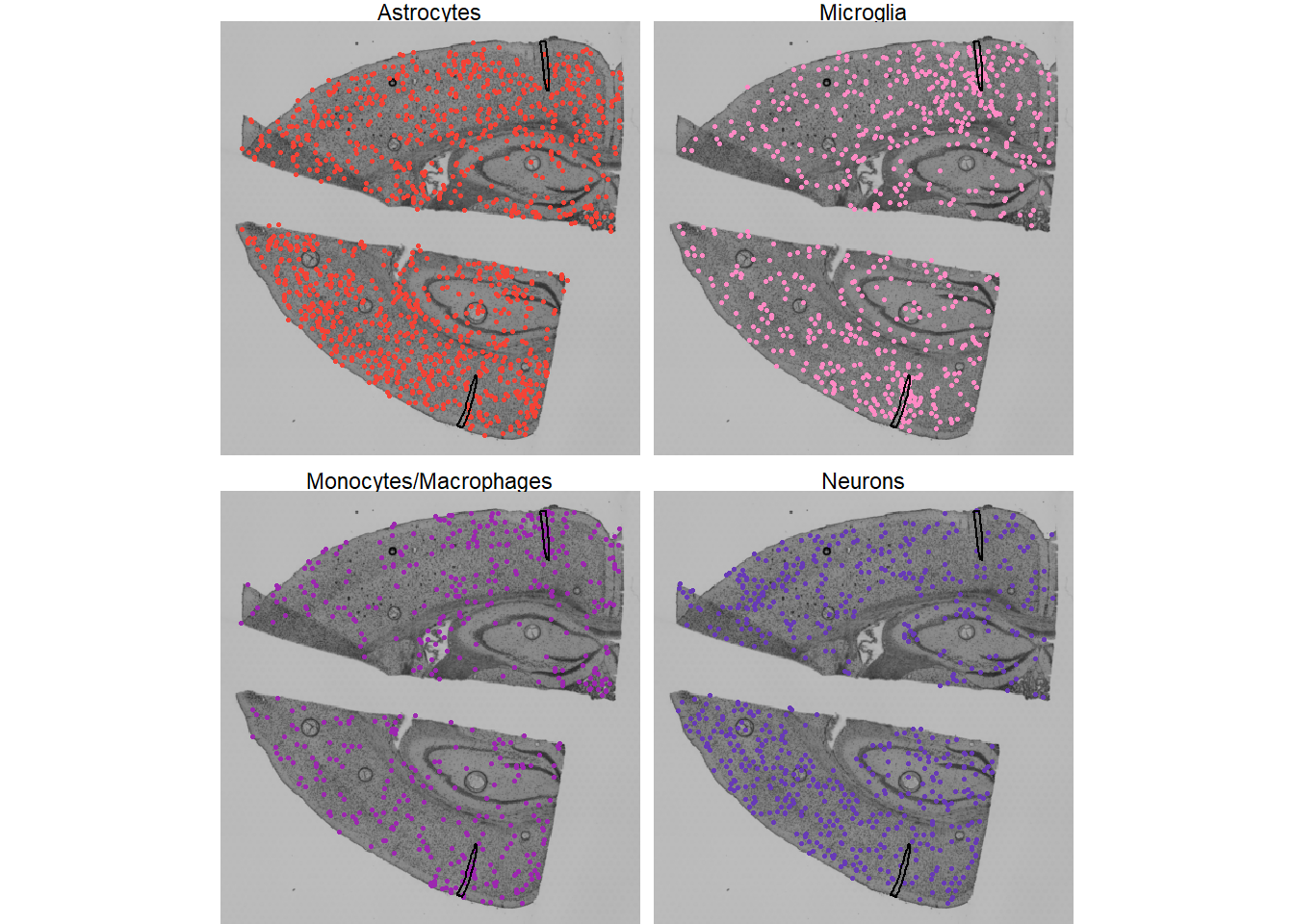
Fig.2 Single cells of different cell types plotted on histology.
2d density plots might be more insightful.
plotSurfaceSC(
  object = object_mci,
  sc_input = sc_mci,
  cell_types = cell_types,
  display_image = TRUE,
  display_density = TRUE,
  display_points = FALSE,
  display_facets = TRUE,
  line_size = 0.5
) +
  injury_add_on_thin +
  legendNone()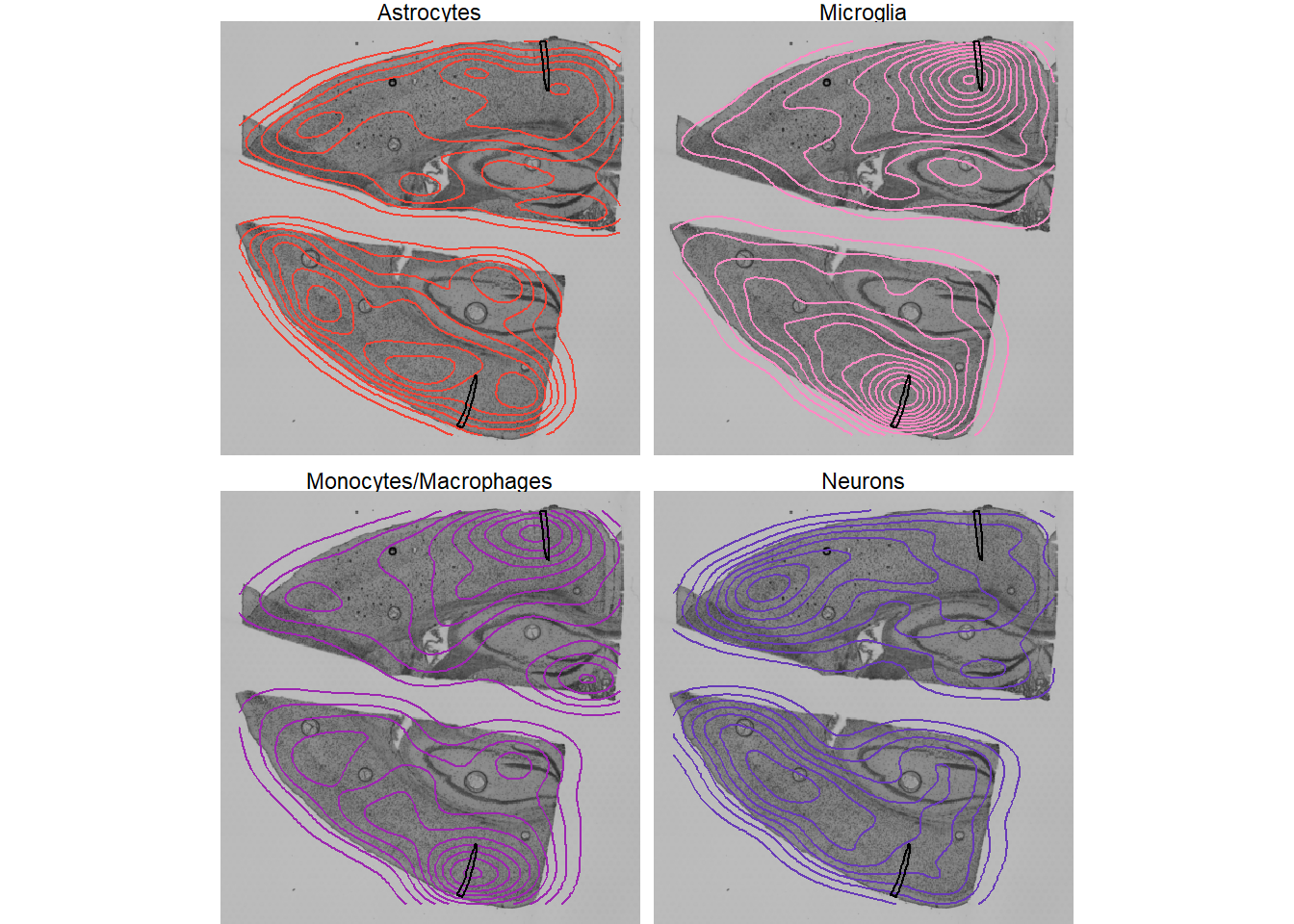
Fig.3 2D kernel density estimates of single cells on the histology.
The density of both, microglia and monocytes, seems to decrease rapidly with the distance to the image annotations. The contrary seems to apply to neurons. The density of astrocytes seems not to be significantly affected.
4. Spatial relation to image annotations
The density of specific cells might stand in relation to the distance to specific areas in the tissue. Figure 3 indicates high density of microglia and monocytes around the injury zones. As we have shown in our vignettes about gene expression and image annotations one can plot the abundance of X against the distance to image annotations, thus specific histological microstructures.
plotImageGgplot(object = object_mci) +
  ggpLayerEncirclingIAS(
    object = object_mci,
    id = c("inj1", "inj2"),
    distance = "1mm"
  ) +
  ggpLayerScaleBarSI(
    object = object_mci,
    sb_dist = "1mm",
    sb_pos = c("1.5mm", "6.75mm"),
    sgmt_size = 0.75,
    text_size = 7.5
) 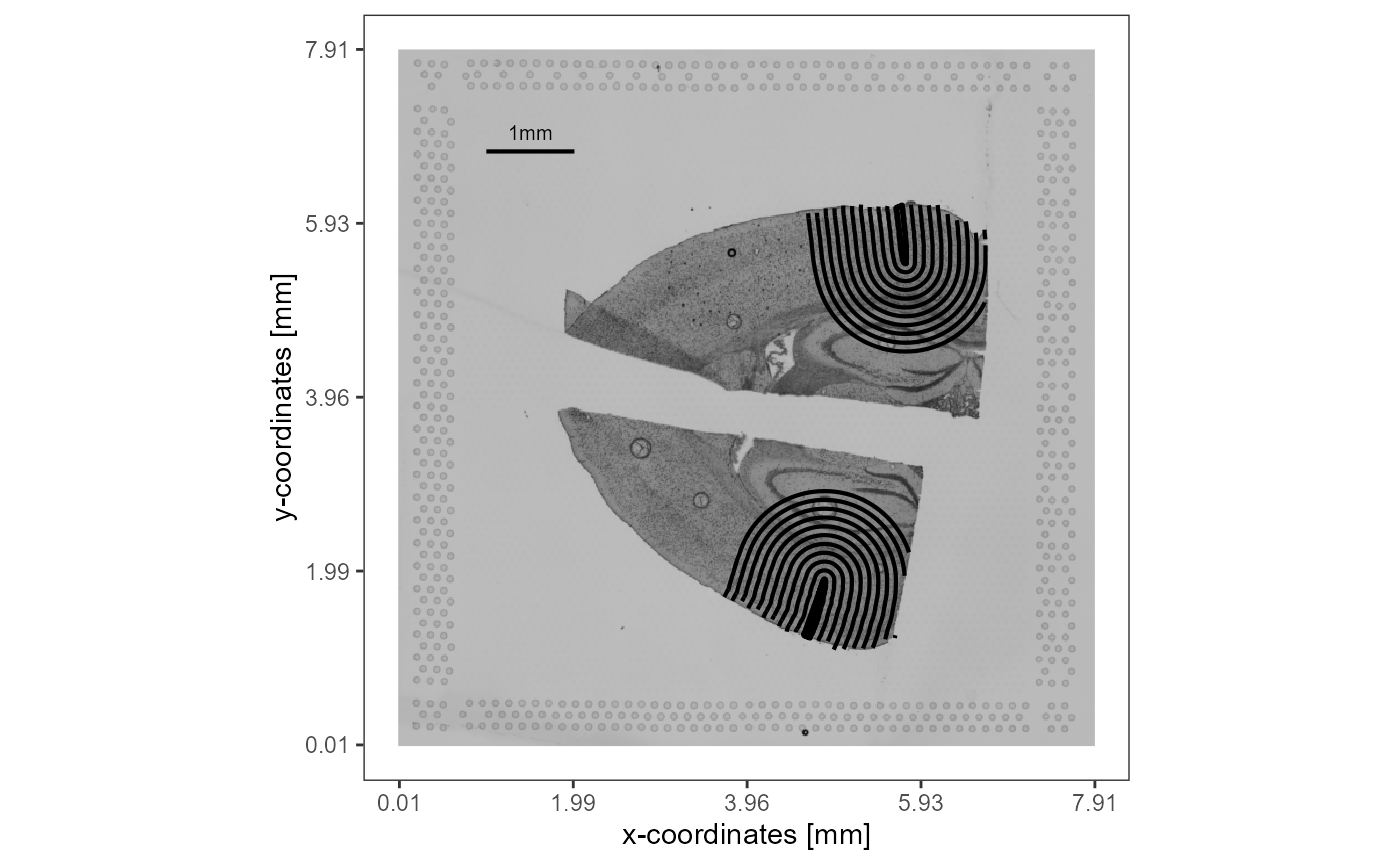
Fig.4 Visualization of the conducted screening of the area around the injury annotations.
Let X be the density of cells.
plotIasRidgeplotSC(
  object = object_mci,
  id = c("inj1", "inj2"), # infer for both and then take the average
  distance = "1mm",
  sc_input = sc_mci,
  free_y = TRUE,
  display_border = TRUE,
  include_area = TRUE # include the area of the injury annotations
) +
  labs(subtitle = "a) Free y-axis") +
  legendNone()

plotIasRidgeplotSC(
  object = object_mci,
  id = c("inj1", "inj2"),
  distance = "1mm",
  sc_input = sc_mci,
  free_y = FALSE,
  display_border = TRUE,
  include_area = TRUE
) +
  labs(subtitle = "b) Fixed y-axis") +
  legendNone()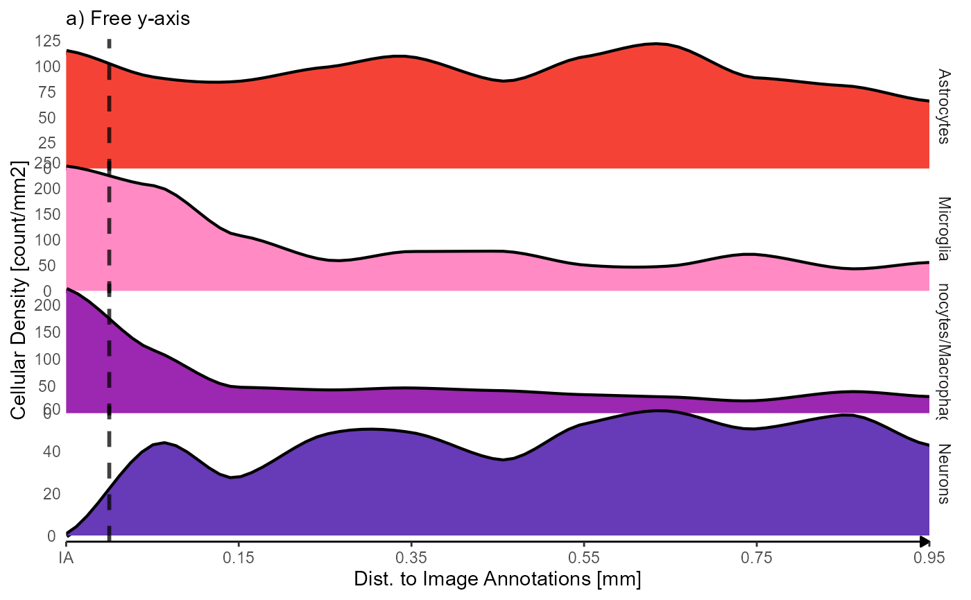
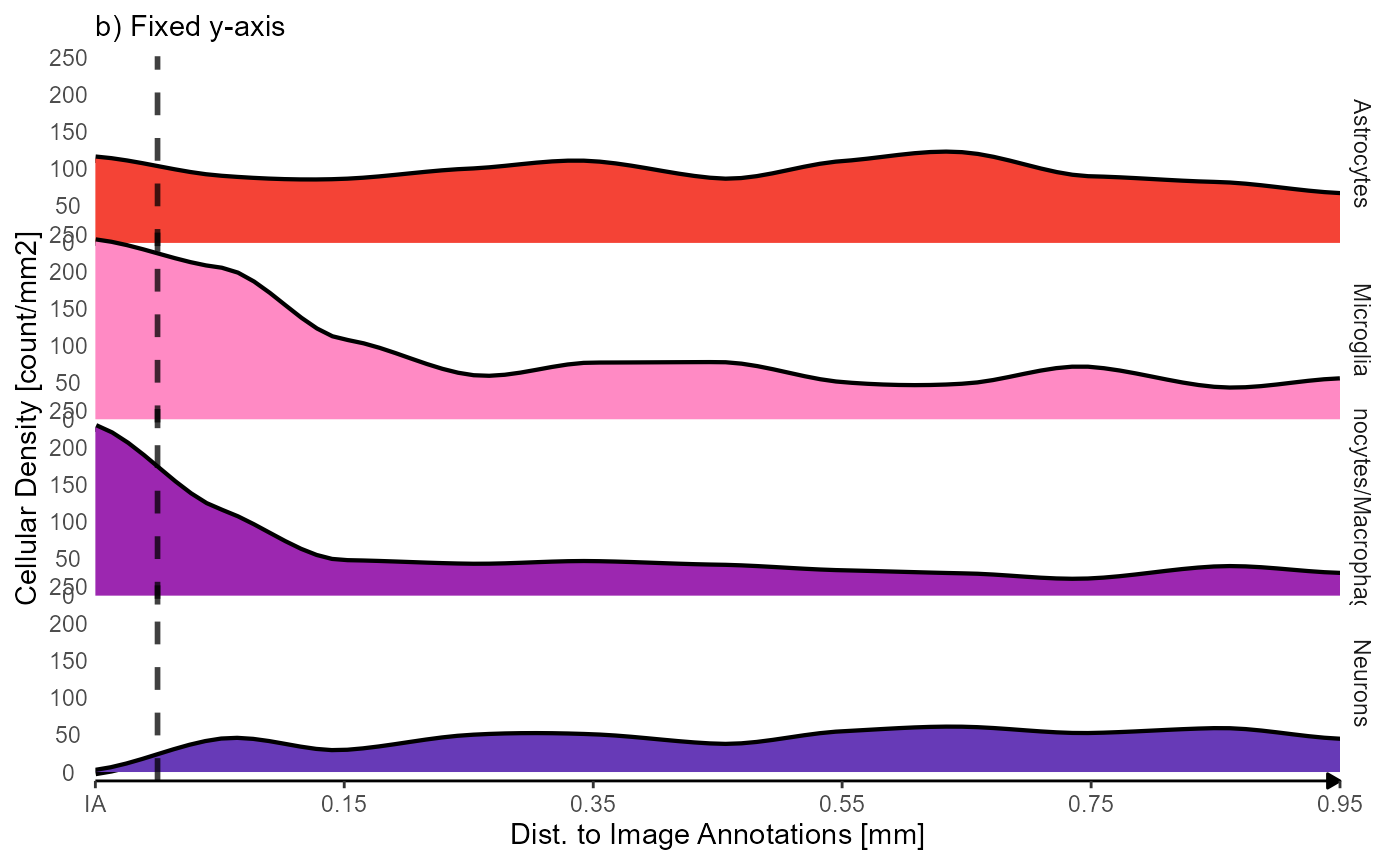
Fig.4 Inferred density of cell types as a function of distance to the injury annotations.
Use the function inferSingleCellGradient() to obtain the
results in a data.frame.
inferSingleCellGradient(
  object = object_mci,
  sc_input = sc_mci,
  id = c("inj1", "inj2"),
  distance = "1mm",
  calculate = "density", # compute density
  area_unit = "mm2", # with unit count/mm2
  normalize = FALSE # do not rescale to 0-1
)
## # A tibble: 11 x 7
## bins_circle bins_order bins_angle Neurons Astrocytes Microglia
## <fct> <dbl> <fct> <dbl> <dbl> <dbl>
## 1 Core 0 (0,360] 0 114. 240.
## 2 Circle 1 1 (0,360] 42.1 87.9 202.
## 3 Circle 2 2 (0,360] 26.9 83.7 105.
## 4 Circle 3 3 (0,360] 47.2 97.4 57.4
## 5 Circle 4 4 (0,360] 48.1 108. 73.7
## 6 Circle 5 5 (0,360] 35.3 84.2 74.3
## 7 Circle 6 6 (0,360] 52.1 108. 47.3
## 8 Circle 7 7 (0,360] 58.2 119. 45.5
## 9 Circle 8 8 (0,360] 49.8 87.0 67.8
## 10 Circle 9 9 (0,360] 56.4 79.5 40.8
## 11 Circle 10 10 (0,360] 42.0 64.4 52.4
## # i 1 more variable: `Monocytes/Macrophages` <dbl>The columns named by the cell type contain the density values
calculated for each distance/circular bin in the unit specified via
area_unit. Use the argument as_models = TRUE
to obtain the results as valid input for add_models in image annotation
screening.
inferSingleCellGradient(
  object = object_mci,
  sc_input = sc_mci,
  id = c("inj1", "inj2"),
  distance = "1mm",
  calculate = "density",
  as_models = TRUE
)
## $Neurons
## [1] 0.0000000 0.7229662 0.4624053 0.8106138 0.8261313 0.6065198 0.8960836
## [8] 1.0000000 0.8564700 0.9695214 0.7225793
##
## $Astrocytes
## [1] 0.9022810 0.4304072 0.3522829 0.6027643 0.7881667 0.3631900 0.7889645
## [8] 1.0000000 0.4141949 0.2756438 0.0000000
##
## $Microglia
## [1] 1.00000000 0.80944945 0.32133099 0.08314482 0.16503405 0.16838363
## [7] 0.03270634 0.02345116 0.13558303 0.00000000 0.05814409
##
## $`Monocytes/Macrophages`
## [1] 1.00000000 0.45156204 0.11913118 0.09565253 0.11272233 0.08934293
## [7] 0.05290540 0.03235082 0.00000000 0.07798454 0.035895465. Accounting for multiple sections
Note that this sample contains two sections that, albeit being from
the same organ, are independent of each other. Relating cells from one
section to the image annotation of another section does not make any
sense. The function add_tissue_section_variable() and
include_tissue_outline() account for that as is exemplified
in this visualization with a distance set to 6mm which would go beyond
the capture frame of the Visium slide.
# visualizes the result of include_tissue_outline()
tissue_outline <-
  ggpLayerTissueOutline(object_mci, line_color = "black", line_size = 1)

# uses include_tissue_outline()
many_expansions <-
  ggpLayerEncirclingIAS(
    object = object_mci,
    id = c("inj1", "inj2"),
    distance = "6mm",
    line_size = 1
    )

ggplot() +
  ggpLayerImage(object_mci) +
  theme_bw() +
  coord_equal() +
  tissue_outline +
  ggpLayerThemeCoords()

ggplot() +
  ggpLayerImage(object_mci) +
  theme_bw() +
  coord_equal() +
  tissue_outline +
  many_expansions +
  ggpLayerThemeCoords()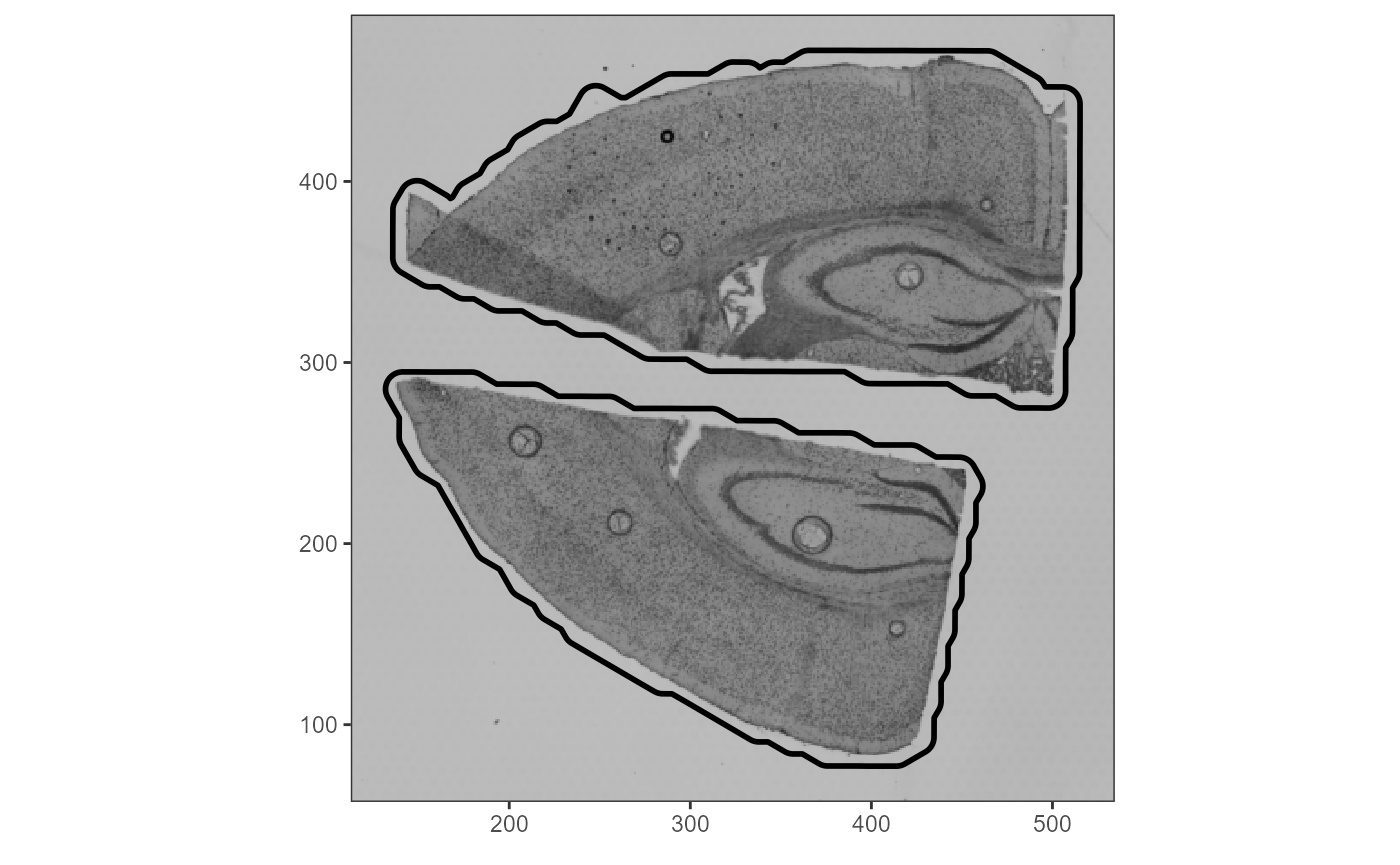
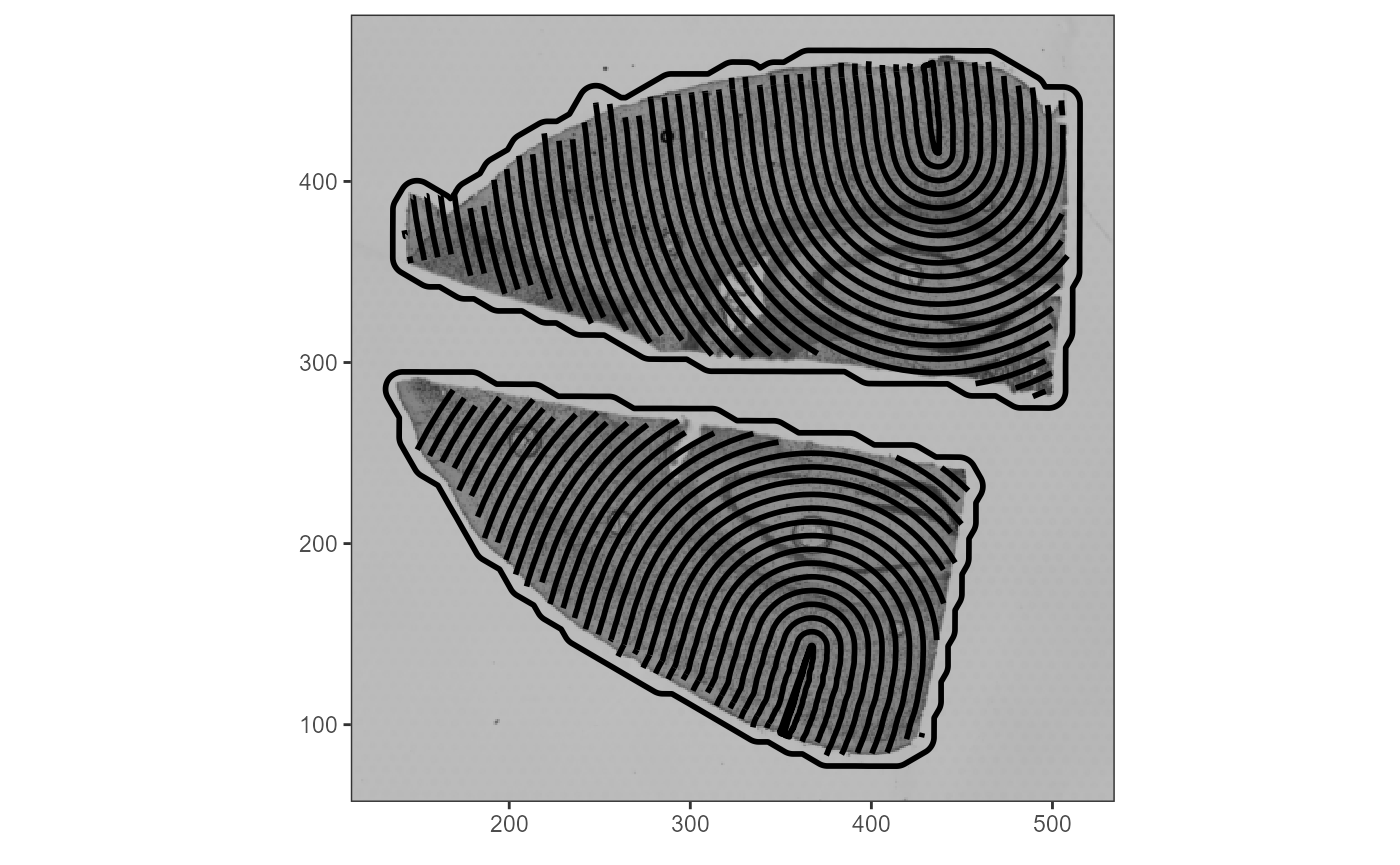
Fig.6 Visualization of how SPATA2 considers the outline of actual tissue sections within algorithms.