Image Handling
spata-v2-image-handling.Rmd2. Introduction
Spatial transcriptomic output comes with a histology image of the dissolved tissue. Apart from visualization of barcode-spot features on the image SPATA2 offers many functions for histology specific analysis. Therefore, detailed interaction between image dimensions and extent and barcode-spot positions in form of data coordinates is required.
This vignette is split in two parts. The first one introduces the basic functions that ensure alignment between image and barcode-spot coordinates and that allow to exchange low- and high resolution image that come with any 10X Visium output.
The second part goes beyond what is necessary to deal with the 10X Visium output and explains in depth how images are stored and dealt with.
3. Basic image handling
The easiest way to load the images of the spatial-folder from the 10X
Visium output in the spata2 object is to use the
initiateSpataObject_10X(). It handles everything. Click here
to download the outs folder of the sample #UKF336, a primary
glioblastoma, which will be used throughout this vignette.
# unzip the downloaded folder and store it under this directory
# (alternatively, change the code and adjust it to the directory of your choice)
directory_to_10X <- "data\\10XVisium\\#UKF336_T_P"

object_t336 <-
  initiateSpataObject_10X(
    directory_10X = directory_to_10X,
    sample_name = "UKF336T",
    image_name = "tissue_lowres_image.png" # defaults to "tissue_lowres_image.png"
  )
3.1 Extracting image data
To obtain the image, that is currently set as well as meta
information there exist several functions prefixed with
getImage*(). To name a few:
# the image
getImage(object_t336)
## Image
##   colorMode    : Color
##   storage.mode : double
##   dim          : 572 600 3
##   frames.total : 3
##   frames.render: 1
##
## imageData(object)[1:5,1:6,1]
##           [,1]      [,2]      [,3]      [,4]      [,5]      [,6]
## [1,] 0.9647059 0.9647059 0.9647059 0.9647059 0.9647059 0.9647059
## [2,] 0.9647059 0.9647059 0.9647059 0.9647059 0.9647059 0.9647059
## [3,] 0.9647059 0.9607843 0.9647059 0.9647059 0.9647059 0.9647059
## [4,] 0.9647059 0.9647059 0.9647059 0.9647059 0.9647059 0.9647059
## [5,] 0.9647059 0.9647059 0.9647059 0.9647059 0.9686275 0.9686275

# image dimensions in width, height and colors
getImageDims(object_t336)
## [1] 572 600   3

# image range in terms of data coordinates
getImageRange(object_t336)
## $x
## [1]   0 572
##
## $y
## [1]   0 600

# directory / object from where the currently set image was read in
getImageOrigin(object_t336)
## [1] "data\\10XVisium\\#UKF336_T_P/spatial/tissue_lowres_image.png"
Normally, image and coordinates are perfectly aligned after reading everything in.
plotSurface(object_t336, pt_alpha = 0.5) +
  ggpLayerThemeCoords(unit = "px")
Fig.1 Image and coordinates are perfectly aligned.
If this is not the case with your sample check out section 4.
Spatial transformations of this vignette to read more about how
SPATA2 deals with spatial linear image transformations.
3.2 High and low resolution
In case of 10X Visium data sets, every spatial folder contains at
least two images usually named tissue_lowres_image.png and
tissue_highres_image.png. A spata2 object only
carries one image at a time. It defaults to read in the low resolution
image. To facilitate switching between high and low resolution image
specific directories can be stored in the spata2 object.
initiateSpataObject_10X() automatically sets the
directories for low resolution and high resolution.
getImageDirLowres(object_t336)## [1] "data\\10XVisium\\#UKF336_T_P/spatial/tissue_lowres_image.png"
getImageDirHighres(object_t336)## [1] "data\\10XVisium\\#UKF336_T_P/spatial/tissue_hires_image.png"The source of the image that is currently read in can be obtained via
getImageOrigin(). To switch between image versions use the
loadImage*() functions.
high_res_obj <- loadImageHighres(object_t336)

high_res_img <- plotSurface(high_res_obj, pt_alpha = 0.5)

low_res_obj <- loadImageLowres(object_t336)

low_res_img <- plotSurface(low_res_obj, pt_alpha = 0.5)

# plot results
high_res_img +
  ggpLayerThemeCoords(unit = "px") +
  labs(subtitle = "High res.")

low_res_img +
  ggpLayerThemeCoords(unit = "px") +
  labs(subtitle = "Low res.")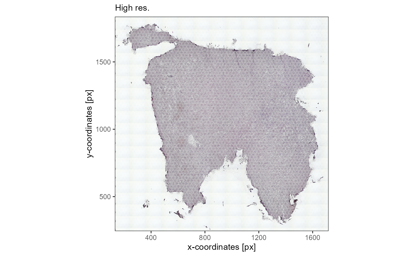
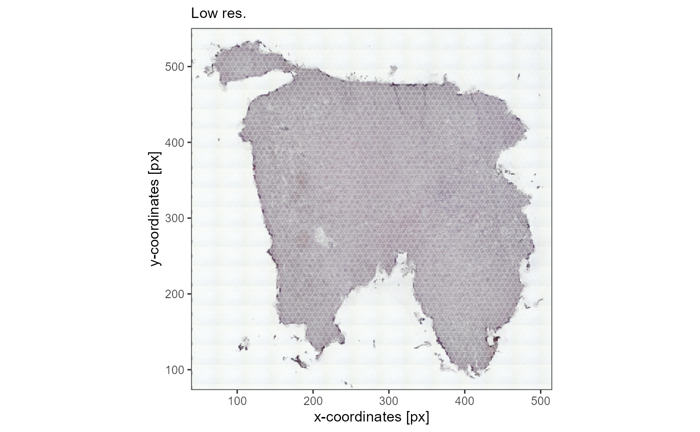
Fig.2 The same image in different resolutions. loadImage*()
takes care of the alignment.
Note: Different image resolutions come with a different number of
pixels. Coordinate based data such as coordinates of the barcode-spots,
spatial trajectories, image annotations etc. have to be scaled and the
pixel scale factor must be
adjusted. The loadImage*() functions do that
automatically!
3.3 Additional images
Different imaging techniques allow to store more than just images of
different resolution. In our example, we imaged the tissue immediately
after surgical extraction with RAMAN spectroscopy. To store directories
of additional images to the images the spata2 objects knows
use the addImageDir() function.
object_t336 <-
  addImageDir(
    object = object_t336,
    dir = file.path(directory_to_10X, "spatial", "raman_tissue_hires_image.tif"),
    name = "raman_spectr" # name of the image with which to refer to it in the future
  )
In general, all directories known to the spata2 object
can be obtained via getImageDirectories().
getImageDirectories(object_t336)## default
## "data\\10XVisium\\#UKF336_T_P/spatial/tissue_lowres_image.png"
## lowres
## "data\\10XVisium\\#UKF336_T_P/spatial/tissue_lowres_image.png"
## highres
## "data\\10XVisium\\#UKF336_T_P/spatial/tissue_hires_image.png"
## raman_spectr
## "C:\\Informatics\\R-Folder\\Packages\\SPATA2\\vignettes\\data\\10XVisium\\#UKF336_T_P/spatial/raman_tissue_hires_image.tif"To use load them as the current background image use
loadImage() and refer to them by name.
object_t336 <- loadImage(object_t336, name = "raman_spectr")

raman_image <-
  plotImageGgplot(
    object = object_t336,
    unit = "mm",
    xrange = c("1.5mm", "6.5mm"),
    yrange = c("1.5mm", "6.5mm")
    ) +
  labs(subtitle = "Image zoomed in")

raman_surface <-
  plotSurface(object_t336, pt_alpha = 0.5) +
  labs(subtitle = "Image with barcode spots")

# plot results
raman_image

raman_surface +
  ggpLayerThemeCoords(unit = "px")+
  labs(subtitle = "RAMAN Spectroscopy")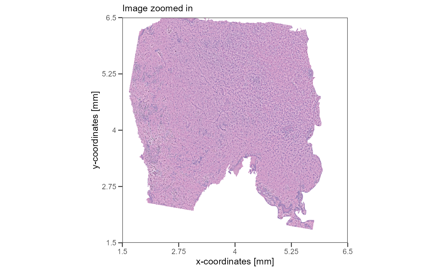
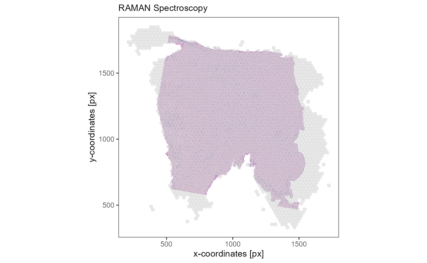
Fig.3 Different images of the same tissue.
To go back to the image you initiated the object with use
loadImageDefault().
object_t336 <- loadImageDefault(object_t336)

getImageOrigin(object_t336)
## [1] "data\\10XVisium\\#UKF336_T_P/spatial/tissue_lowres_image.png"4. Spatial transformations
To align image and barcode-spot coordinates spatial transformations such as flipping, rotating and scaling might become necessary.
4.1 Applying transformation of images
To align an image with coordinates spatial transformation can become
necessary. The flipImage(), rotateImage()
functions do that. Note that the
<transformation>Image() functions only affect the
image! In case of already aligned image and coordinates a simple call to
<transformation>Image() interferes with the
alignment.
4.1.1 Flipping
To show the usage of flipImage() we read in a badly
aligned image. Note that exchangeImage() is the working
horse behind all loadImage*() functions. It reads in the
image and performs all the necessary transformation and scaling step to
keep image and coordinates aligned.
# create bad alignment manually
object_t336_flipped_bad <-
  exchangeImage(
    object = object_t336,
    image = str_c(directory_to_10X, "\\spatial\\tissue_lowres_image_bad_alignment_flipped.png")
    )

# image is flipped and not aligned with coordinates
plotSurface(object_t336_flipped_bad, pt_alpha = 0.5) +
  ggpLayerThemeCoords(unit = "px")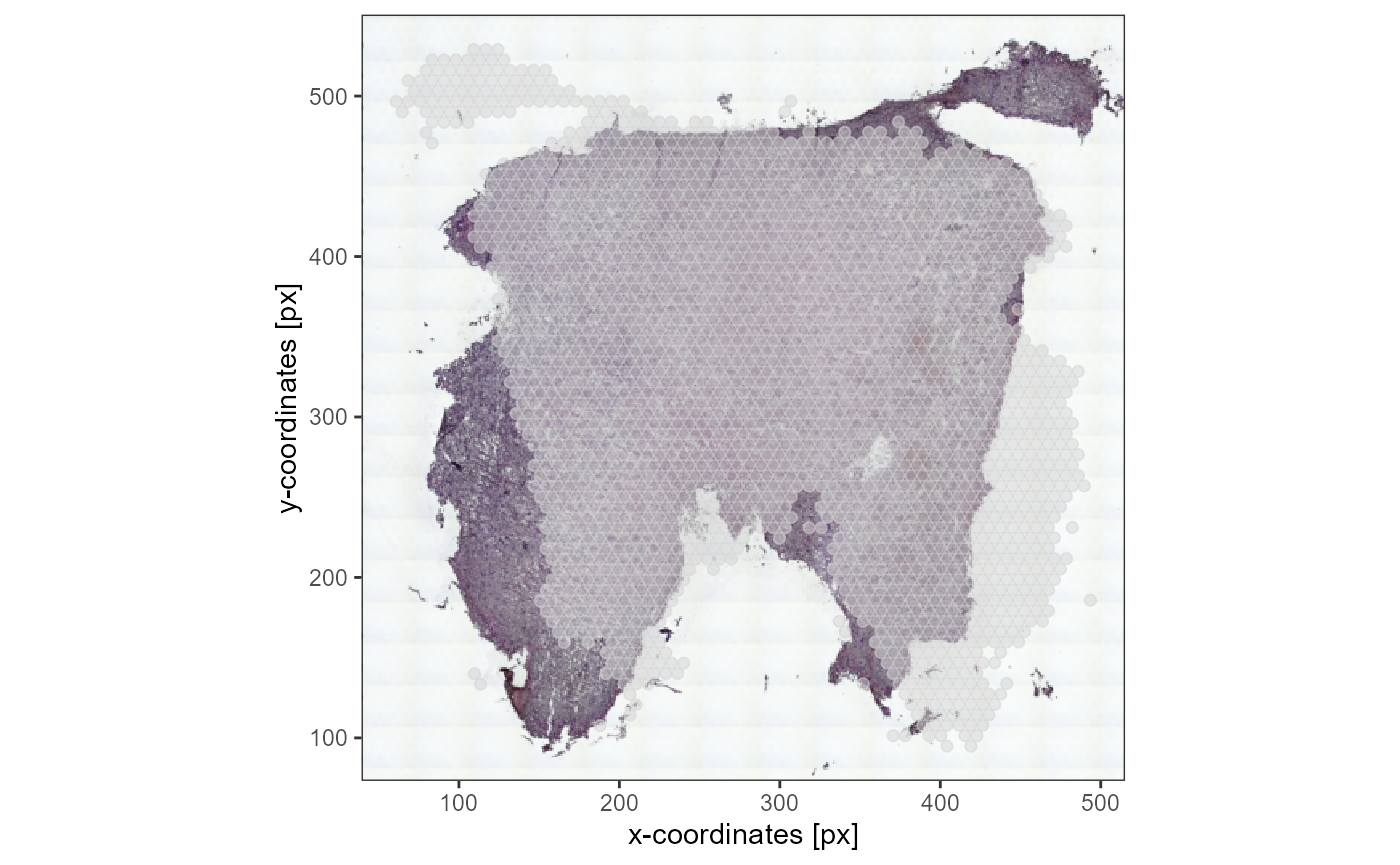
Fig.4 Image is not aligned with coordinates and must be flipped along the vertical axis.
Applying flipImage() on a bad aligned image fixes the
alignment.
object_t336_flipped_fixed <-
  flipImage(
    object = object_t336_flipped_bad,
    axis = "vertical"
    )

plotSurface(object_t336_flipped_fixed, pt_alpha = 0.5) +
  ggpLayerThemeCoords(unit = "px")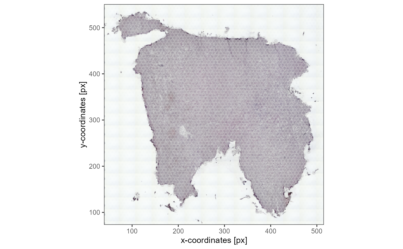
Fig.5 Image and coordinates are aligned after spatial transformation.
4.2 Spatial transformation of the whole object
Assuming that image and coordinates are aligned you do
not want to use flipImage() to change the
justification of the surface plots as flipImage() only
flips the image and lets spatial aspects as they are. To transform image
and coordinates alike use flipAll(),
rotateAll() and scaleAll().
object_t336_flipped <- flipAll(object = object_t336, axis = "horizontal")

plotSurface(object_t336_flipped, pt_alpha = 0.5) +
  ggpLayerThemeCoords(unit = "px")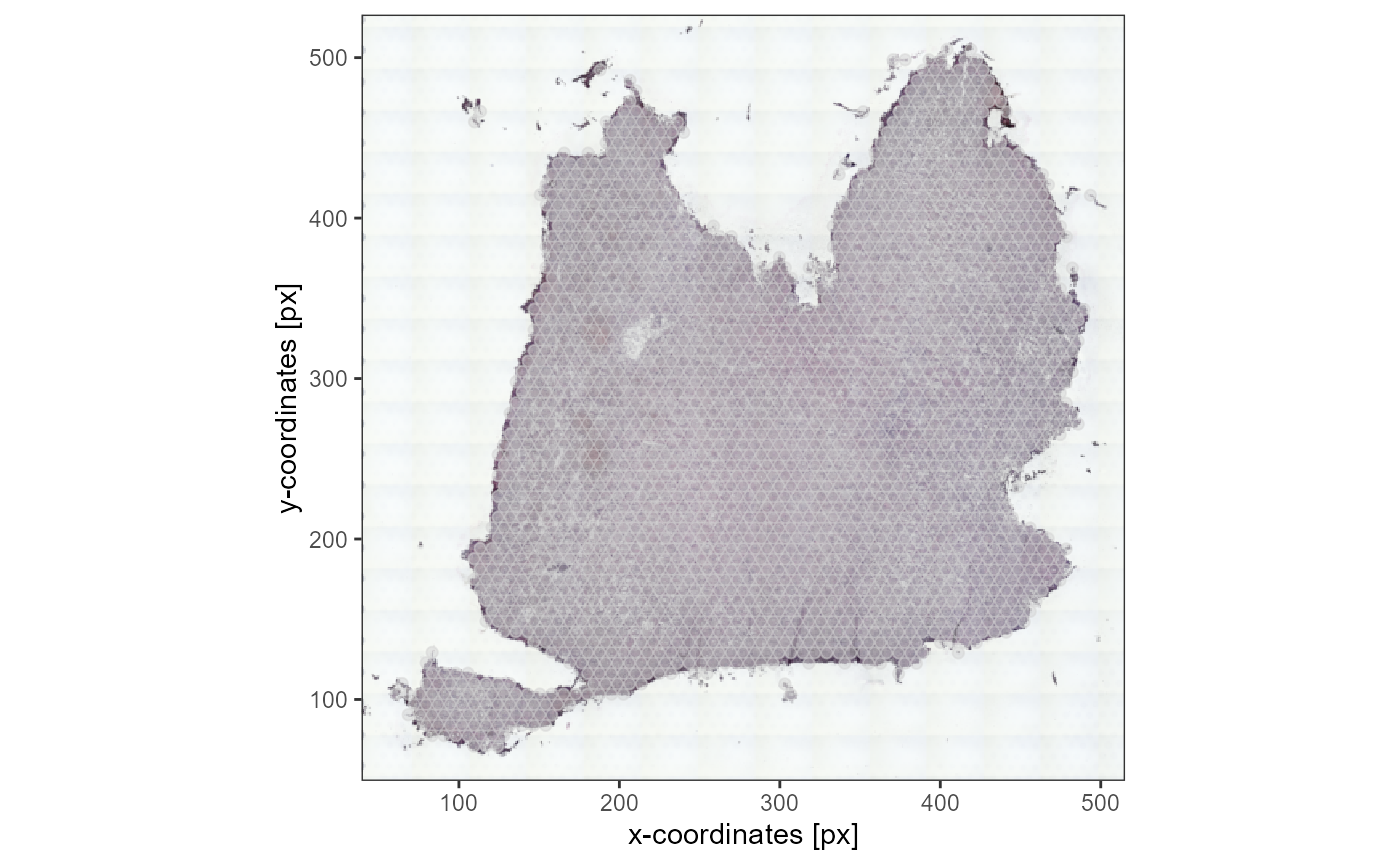
Fig.9 The whole dataset is flipped.
4.3 Tracking transformation of images
Changes in justification of the whole object are tracked. After
initiation of the spata2 object the justification should
look like this.
# default justification
getImageInfo(object_t336)
## $dim_input
## [1] 572 600 3
##
## $dim_stored
## [1] 572 600 3
##
## $img_scale_fct
## [1] 1
##
## $origin
## [1] "data\\10XVisium\\#UKF336_T_P/spatial/tissue_lowres_image.png"
##
## $angle
## [1] 0
##
## $flipped
## $flipped$horizontal
## [1] FALSE
##
## $flipped$vertical
## [1] FALSEAfter performing spatial transformations it is tracked how the current state of the object deviates from the starting default.
object_t336_flipped <- flipAll(object_t336, axis = "horizontal")

img_obj_flipped <- getImageObject(object_t336_flipped)

getImageInfo(object_t336_flipped)
## $dim_input
## [1] 572 600 3
##
## $dim_stored
## [1] 572 600 3
##
## $img_scale_fct
## [1] 1
##
## $origin
## [1] "data\\10XVisium\\#UKF336_T_P/spatial/tissue_lowres_image.png"
##
## $angle
## [1] 0
##
## $flipped
## $flipped$horizontal
## [1] TRUE
##
## $flipped$vertical
## [1] FALSEAssuming that all images that belong to the tissue are stored with the same justification the justification state of the object can be compared to the image that should replace the current image and it can be adjusted automatically.
#
object_t336_flipped_low_res <-
  loadImageLowres(
    object = object_t336_flipped,
    adjust = TRUE # defaults to TRUE. Set to FALSE if you don't want automatic adjustment
    )

# object image and coordinates remain flipped
plotSurface(object_t336_flipped_low_res, pt_alpha = 0.5) +
  ggpLayerThemeCoords(unit = "px")
Fig.10 The loaded image has been automatically adjusted by flipping it.
4.4 Ensuring alignment between image and coordinate based aspects
Tracking changes in image justification is necessary, for instance, as coordinate based spatial aspects such as image annotations or spatial trajectories need to know in how far the current image deviates from their parent image in terms of justification and size.
data("image_annotations")

img_ann_mt <- image_annotations$`336_T`$missing_tissue

img_ann_mt@id
## [1] "missing_tissue"

# image annotations contain information regarding how and where they were drawn
img_ann_mt@info
## $parent_id
## [1] "UKF336T"
##
## $parent_origin
## [1] "data\\Visium10X\\#UKF336_T_P\\outs/spatial/tissue_hires_image.png"
##
## $current_dim
## [1] 1908 2000
##
## $current_just
## $current_just$angle
## [1] 0
##
## $current_just$flipped
## $current_just$flipped$horizontal
## [1] TRUE
##
## $current_just$flipped$vertical
## [1] FALSE

object_t336 <- loadImageHighres(object_t336)
The image annotation was drawn on the high resolution version of the
image and it was neither flipped nor rotated. Currently the
spata2 object contains a flipped version of the low
resolution image as is displayed below. While the image annotation is
set its properties are compared to the current image and adjusted in
terms of justification and scale.
object_t336_not_aligned <-
  setImageAnnotation(
    object = object_t336,
    img_ann = img_ann_mt,
    align = FALSE # no alignment
  )

# that seems wrong
no_alignment <-
  plotImageGgplot(object_t336_not_aligned, unit = "px")+
  ggpLayerImgAnnOutline(object = object_t336_not_aligned, ids = "missing_tissue") +
  # allow plotting of observations outside of the tissue frame
  coord_fixed(xlim = NULL, ylim = NULL) +
  labs(subtitle = "No alignment")

object_t336_aligned <-
  setImageAnnotation(
    object = object_t336,
    img_ann = img_ann_mt,
    align = TRUE, # the default
    overwrite = TRUE
  )

# that seems wrong
with_alignment <-
  plotImageGgplot(object_t336_aligned, unit = "px")+
  ggpLayerImgAnnOutline(object = object_t336_aligned, ids = "missing_tissue") +
  coord_fixed(xlim = NULL, ylim = NULL) +
  labs(subtitle = "With alignment")

# plot results
no_alignment
with_alignment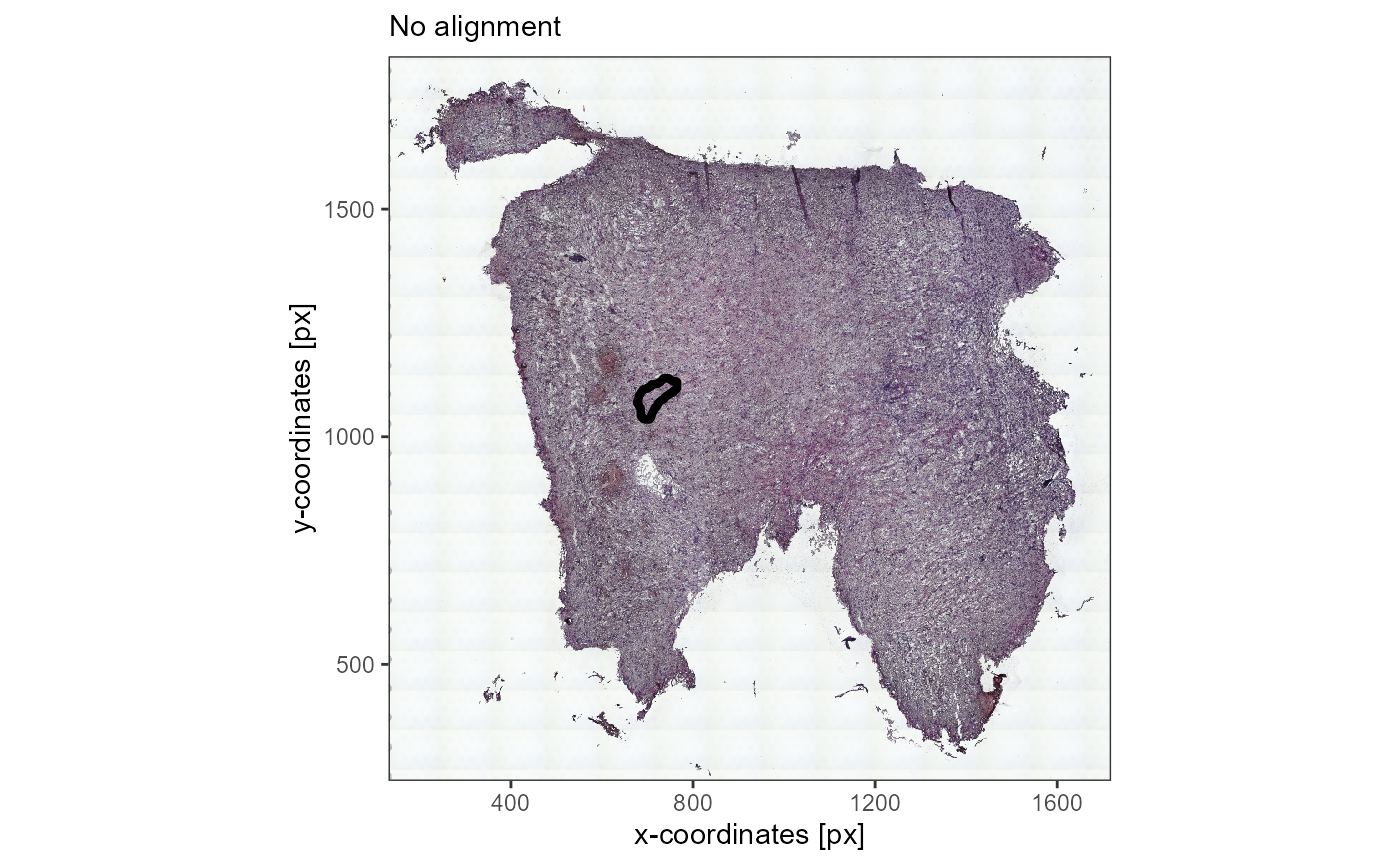
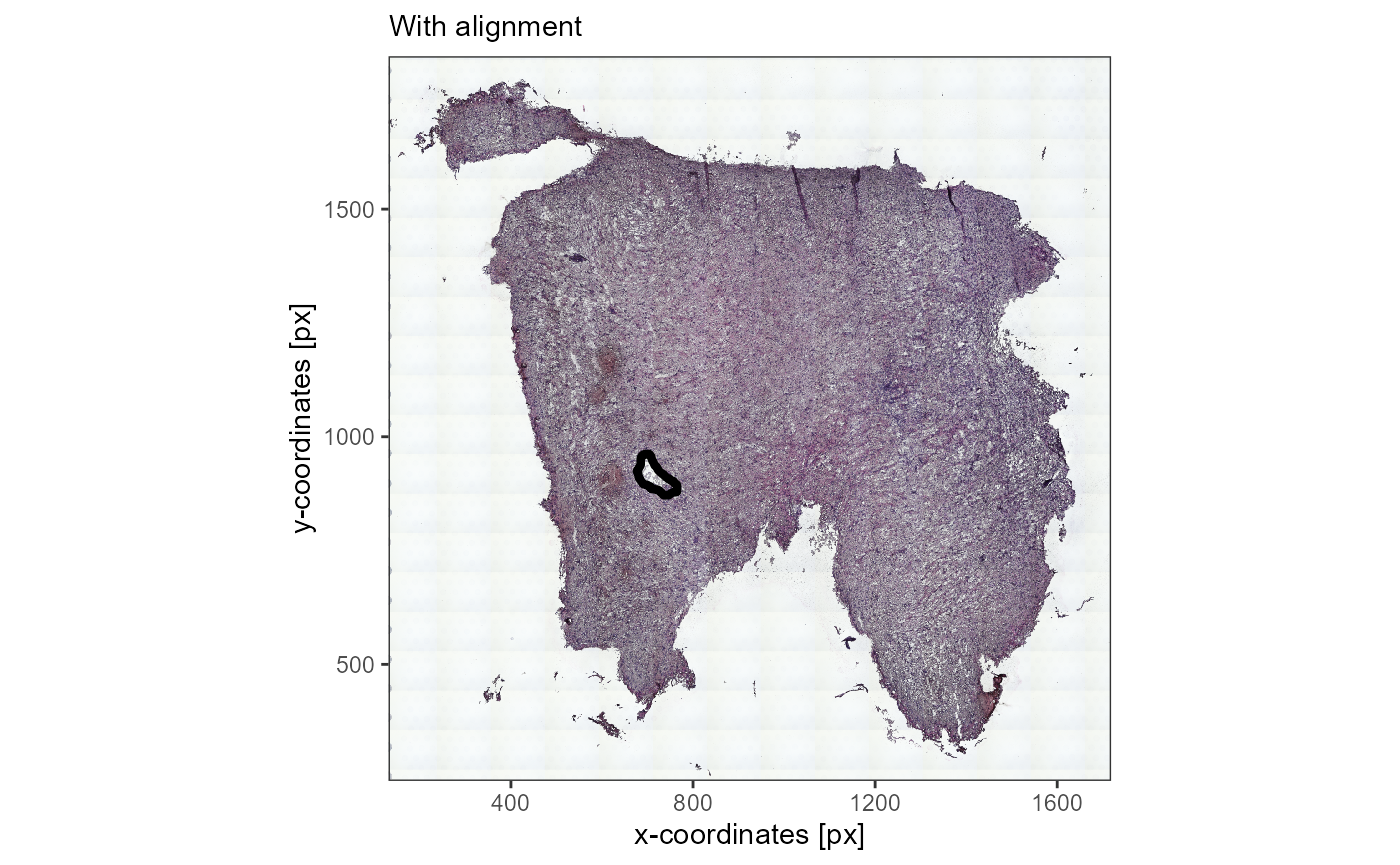
Fig.11 Image annotation that is added is automatically adjusted to changes in image justification.
5. The image container
The S4 object in which data regarding the imaging of the tissue is
stored is an object of class HistologyImaging. It contains
several slots. Run ?HistologyImaging to find extensive
documentation about what each slot is about.
hist_img <- HistologyImaging()

slotNames(hist_img)
## [1] "annotations" "coordinates" "dir_default" "dir_highres"
## [5] "dir_lowres" "dir_add" "grid" "id"
## [9] "image" "image_info" "justification" "meta"
## [13] "misc"The whole object can be obtained via getImageObject().
(Not to confuse with getImage() which only extracts the
image itself.)
io <- getImageObject(object_t336)

str(io)
## Formal class 'HistologyImaging' [package "SPATA2"] with 13 slots
## ..@ annotations : list()
## ..@ coordinates : tibble [2,280 x 11] (S3: tbl_df/tbl/data.frame)
## .. ..$ barcodes: chr [1:2280] "AAACACCAATAACTGC-1" "AAACAGAGCGACTCCT-1" "AAACAGGGTCTATATT-1" "AAACCGGGTAGGTACC-1" ...
## .. ..$ x : num [1:2280] 1510 576 1584 1397 1223 ...
## .. ..$ y : num [1:2280] 554 1526 814 922 705 ...
## .. ..$ tissue : int [1:2280] 1 1 1 1 1 1 1 1 1 1 ...
## .. ..$ row : num [1:2280] 1800 1950 1840 1857 1823 ...
## .. ..$ col : num [1:2280] 60 310.2 40 90.1 136.8 ...
## .. ..$ imagerow: num [1:2280] -36453 -10610 -29553 -26683 -32437 ...
## .. ..$ imagecol: num [1:2280] 40148 15327 42126 37163 32539 ...
## .. ..$ sample : chr [1:2280] "UKF336T" "UKF336T" "UKF336T" "UKF336T" ...
## .. ..$ section : chr [1:2280] "1" "1" "1" "1" ...
## .. ..$ outline : logi [1:2280] TRUE FALSE TRUE FALSE FALSE FALSE ...
## ..@ dir_default : chr "data\\10XVisium\\#UKF336_T_P/spatial/tissue_lowres_image.png"
## ..@ dir_highres : chr "data\\10XVisium\\#UKF336_T_P/spatial/tissue_hires_image.png"
## ..@ dir_lowres : chr "data\\10XVisium\\#UKF336_T_P/spatial/tissue_lowres_image.png"
## ..@ dir_add :List of 1
## .. ..$ raman_spectr: chr "C:\\Informatics\\R-Folder\\Packages\\SPATA2\\vignettes\\data\\10XVisium\\#UKF336_T_P/spatial/raman_tissue_hires_image.tif"
## ..@ grid : list()
## ..@ id : chr "UKF336T"
## ..@ image :Formal class 'Image' [package "EBImage"] with 2 slots
## .. .. ..@ .Data : num [1:1908, 1:2000, 1:3] 0.965 0.961 0.965 0.965 0.965 ...
## .. .. ..@ colormode: int 2
## .. .. ..$ dim: int [1:3] 1908 2000 3
## ..@ image_info :List of 4
## .. ..$ dim_input : int [1:3] 1908 2000 3
## .. ..$ dim_stored : int [1:3] 1908 2000 3
## .. ..$ img_scale_fct: num 1
## .. ..$ origin : chr "data\\10XVisium\\#UKF336_T_P/spatial/tissue_hires_image.png"
## ..@ justification:List of 2
## .. ..$ angle : num 0
## .. ..$ flipped:List of 2
## .. .. ..$ horizontal: logi FALSE
## .. .. ..$ vertical : logi FALSE
## ..@ meta : list()
## ..@ misc :List of 1
## .. ..$ VisiumV1:List of 5
## .. .. ..$ origin : chr "VisiumV1"
## .. .. ..$ scale.factors:List of 4
## .. .. .. ..$ spot : num 0.125
## .. .. .. ..$ fiducial: num 208
## .. .. .. ..$ hires : num 0.125
## .. .. .. ..$ lowres : num 0.0376
## .. .. .. ..- attr(*, "class")= chr "scalefactors"
## .. .. ..$ assay : chr "Spatial"
## .. .. ..$ spot.radius : num 0.013
## .. .. ..$ key : chr "slice1_"
## ..$ scale_factors: list()