Autoencoder Denoising
spata-v2-autoencoder.Rmd1. Introduction
Sequencing data from single-cell RNA sequencing (scRNA-seq) and from spatial transcriptomic experiments alike are prone to noise and technical artifacts that might obstruct downstram analysis. As recently proposed by Gökcen et al., 2019 autoencoder networks work against that. SPATA2 offers a similar approach to denoise data. Apart from data that makes more sense (see Figure 3.2 and 3.3) denoising your data often results in more insightful visualization.
library(SPATA2)
library(SPATAData)

spata_obj <- downloadSpataObject("275_T")
Note: Before you use the functions SPATA2 provides
please make sure that the R-packages keras and
tensorflow are installed on your device. Installing both
packages requires some steps in addition to what R does by default.
Therefore the installation of SPATA2 does not include
these two packages. Click here
for a guide on how to setup both packages.
2. Denoising your data
Although there es only one function needed to denoise your data,
namely runAutoencoderDenoising(), you might want to assess
how you set up the neural network that does the denoising - see chapter
2.2 for that matter.
2.1 Using the neural network
Denoising your data in SPATA2 is as simple as it
gets. The function runAutoenconderDenoising() constructs
the neural network according to your adjustments (see Chapter 2.2 on how
to optimize that) and stores the resulting denoised expression matrix
named denoised next to the already existing expression matrix
named scaled by using the function
addExpressionMatrix().
# all expression matrices before denoising
getExpressionMatrixNames(object = spata_obj)

# active expression matrix before denoising
getActiveMatrixName(object = spata_obj)
## [1] "scaled"## [1] "scaled"
# denoising your data
spata_obj <-
  runAutoencoderDenoising(
    object = spata_obj,
    activation = "selu",
    bottleneck = 56,
    epochs = 20,
    layers = c(128, 64, 32),
    dropout = 0.1
    )

# all expression matrices after denoising
getExpressionMatrixNames(object = spata_obj)

# active expression matrix after denoising
getActiveMatrixName(object = spata_obj)
## [1] "scaled" "denoised"## [1] "denoised"Use printAutoencoderSummary() if you want to recall the
way you set up the neural network that denoised your scaled data.
# print a summary
printAutoencoderSummary(object = spata_obj)
## The neural network that generated matrix 'denoised' was constructed with the following adjustments:
##
## Activation function: selu
## Bottleneck neurons: 56
## Dropout: 0.1
## Epochs: 20
## Layers: 128, 64 and 32By default all functions in SPATA2 (like
plotSurface() for example) use the expression matrix that
is set to the active expression matrix. Use
setActiveMatrix() to switch between the expression matrices
that are currently stored inside your spata-object.
2.2 The optimal neural network set up
How neural networks are set up and how they work in detail is beyond
the scope of this tutorial. Among other things they differ in the number
of bottleneck neurons as well as in the activation
function they use. With runAutoencoderAssessment() you
can iterate over all combinations you are interested in and assess the
results by the total variance of the principal component analysis
results.
spata_obj <-
  runAutoencoderAssessment(
    object = spata_obj,
    activations = c("relu", "selu", "sigmoid"),
    bottlenecks = c(32, 40, 48, 56, 64),
    epochs = 20,
    layers = c(128, 64, 32),
    dropout = 0.1
    )

plotAutoencoderAssessment(object = spata_obj)
## Additional set up of neural network:
##
## Epochs: 20
## Dropout: 0.1
## Layers: 128, 64 and 32-invis-1.png)
Figure 2.1 Visualization of total variance of different autoencoder set ups
Sticking to the set up that resulted in the highest total variance is
a good start. If you want to extract the assessment results use
getAutoencoderAssessment(). It returns a list of the total
variance results as well as the components the neural networks were
composed of.
3.3 Storing several expression matrices
You can store as many denoised expression matrices as you want in
your spata-object. Use the argument mtr_name_output for
that matter. This makes runAutoencoderDenoising() add the
denoised expression matrix under the name you specified instead of the
default name denoised. Keep in mind that the size of your
spata-object is mainly determined by the data matrices it contains and
that it can quickly grow to several gigabytes which might considerably
affect the speed with which your R session runs.
3. Examples
Figure 3.1 exemplifies how autoencoder denoising captures the main pattern and how this pattern is emphasized in the surface plot using the expression of gene MARCH6.
spata_obj <- setActiveMatrix(object = spata_obj, mtr_name = "scaled")

plotSurface(
  object = spata_obj,
  color_by = "MARCH6",
  pt_size = 1.8
) +
  labs(title = "Scaled (not denoised)") +
  legendNone()

spata_obj <- setActiveMatrix(object = spata_obj, mtr_name = "denoised")

plotSurface(
  object = spata_obj,
  color_by = "MARCH6",
  pt_size = 1.8
  ) +
  labs(title = "Denoised")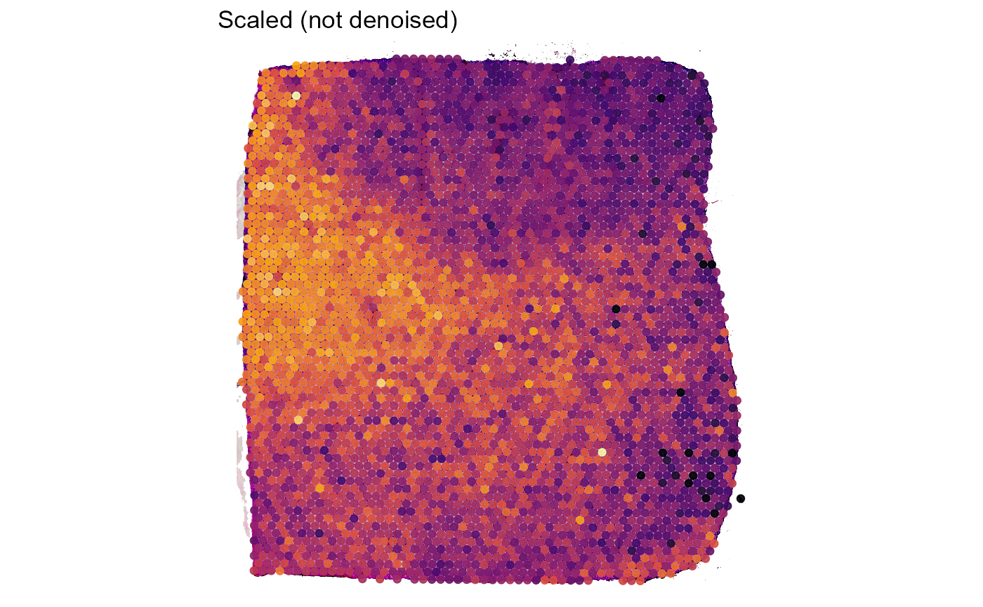
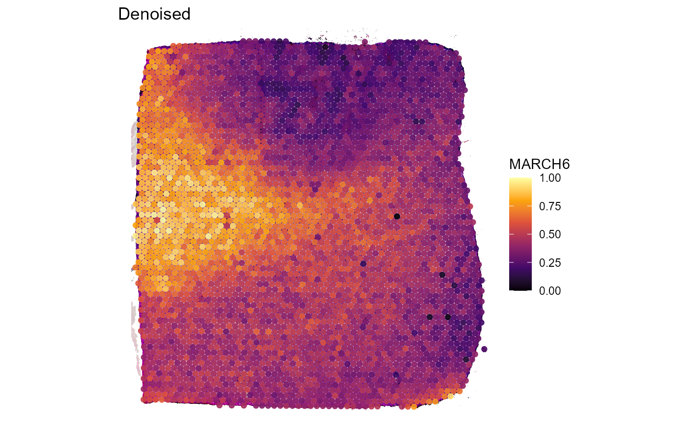
Figure 3.1 First visual demonstration of scaled vs. denoised data
Both, Figure 3.2 and Figure 3.3 go one step further. The example genes AIF1 and CD68 are both expressed in macrophages which, logically, should result in an almost perfect spatial overlap of both genes. Still, technical artifacts might interfere.
example_genes <- c("AIF1", "CD68")

spata_obj <- setActiveMatrix(object = spata_obj, mtr_name = "scaled")

plotSurface(
  object = spata_obj,
  color_by = example_genes[1],
  smooth = FALSE,
  pt_size = 1.8
  ) +
  labs(title = "Scaled (not denoised)")

plotSurface(
  object = spata_obj,
  color_by = example_genes[2],
  smooth = FALSE,
  pt_size = 1.8
  ) +
  labs(title = "Scaled (not denoised)")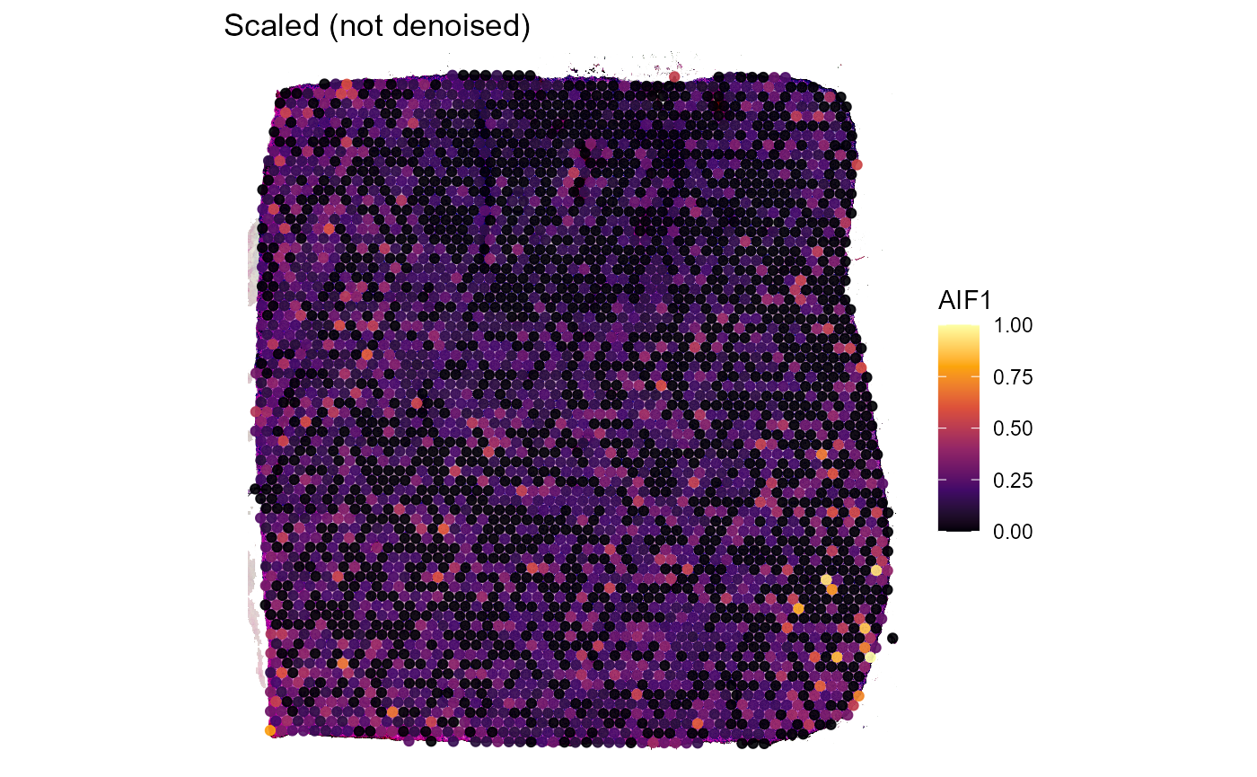
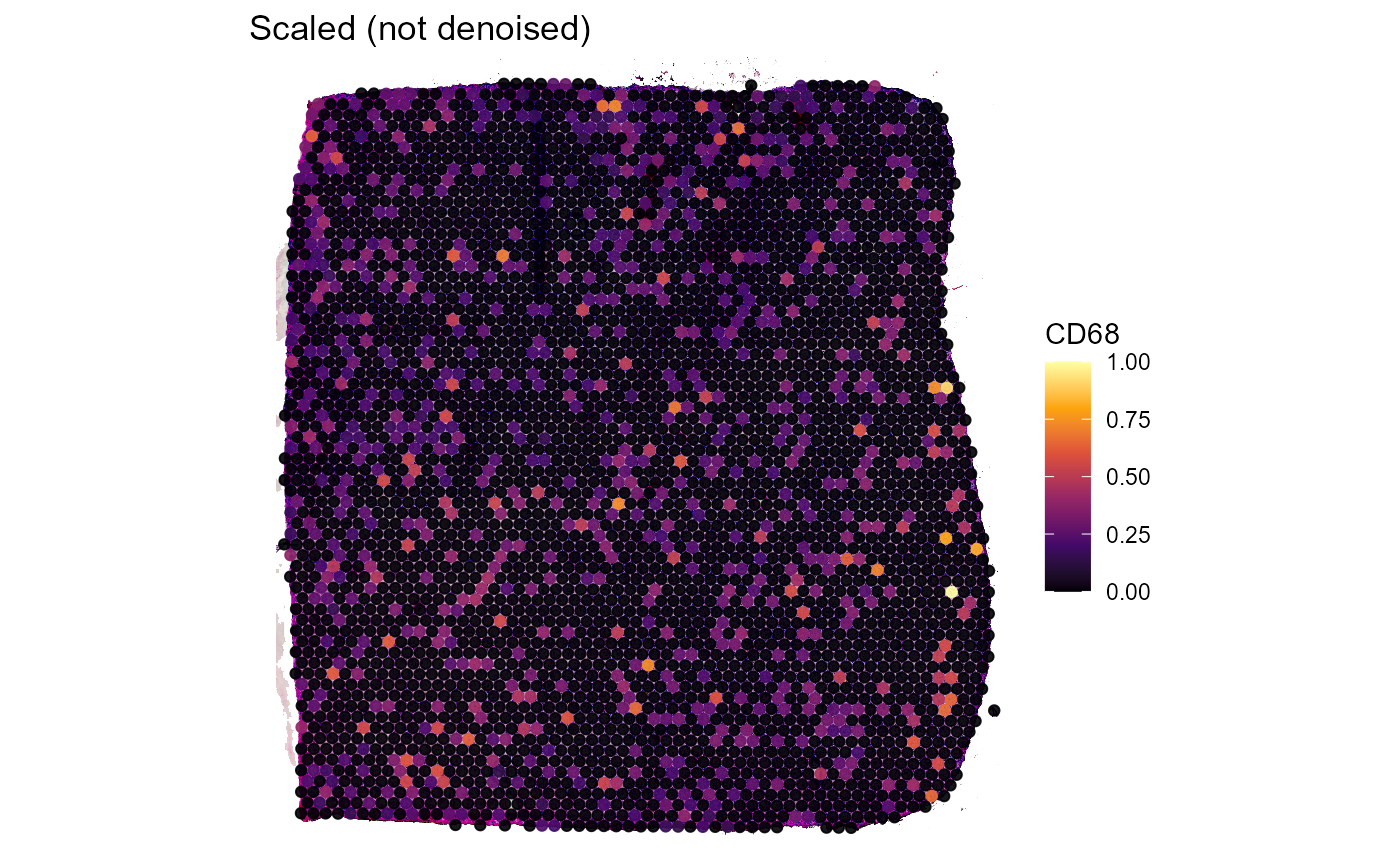
Figure 3.2 Not denoised expression of genes AIF1 and CD68
In addition to that, the fact that both genes naturally differ in expression levels might affect the colors used to represent these expression levels which additionally obscure the exclusive coexpression of AIF1 and CD68 on the same cells. Denoising does not lead to perfectly matching expression but it does a sufficient job in capturing the underlying pattern.
spata_obj <- setActiveMatrix(object = spata_obj, mtr_name = "denoised")

plotSurface(
  object = spata_obj,
  color_by = example_genes[1],
  smooth = FALSE,
  pt_size = 1.8
  ) +
  labs(title = "Denoised")

plotSurface(
  object = spata_obj,
  color_by = example_genes[2],
  smooth = FALSE,
  pt_size = 1.8
  ) +
  labs(title = "Denoised")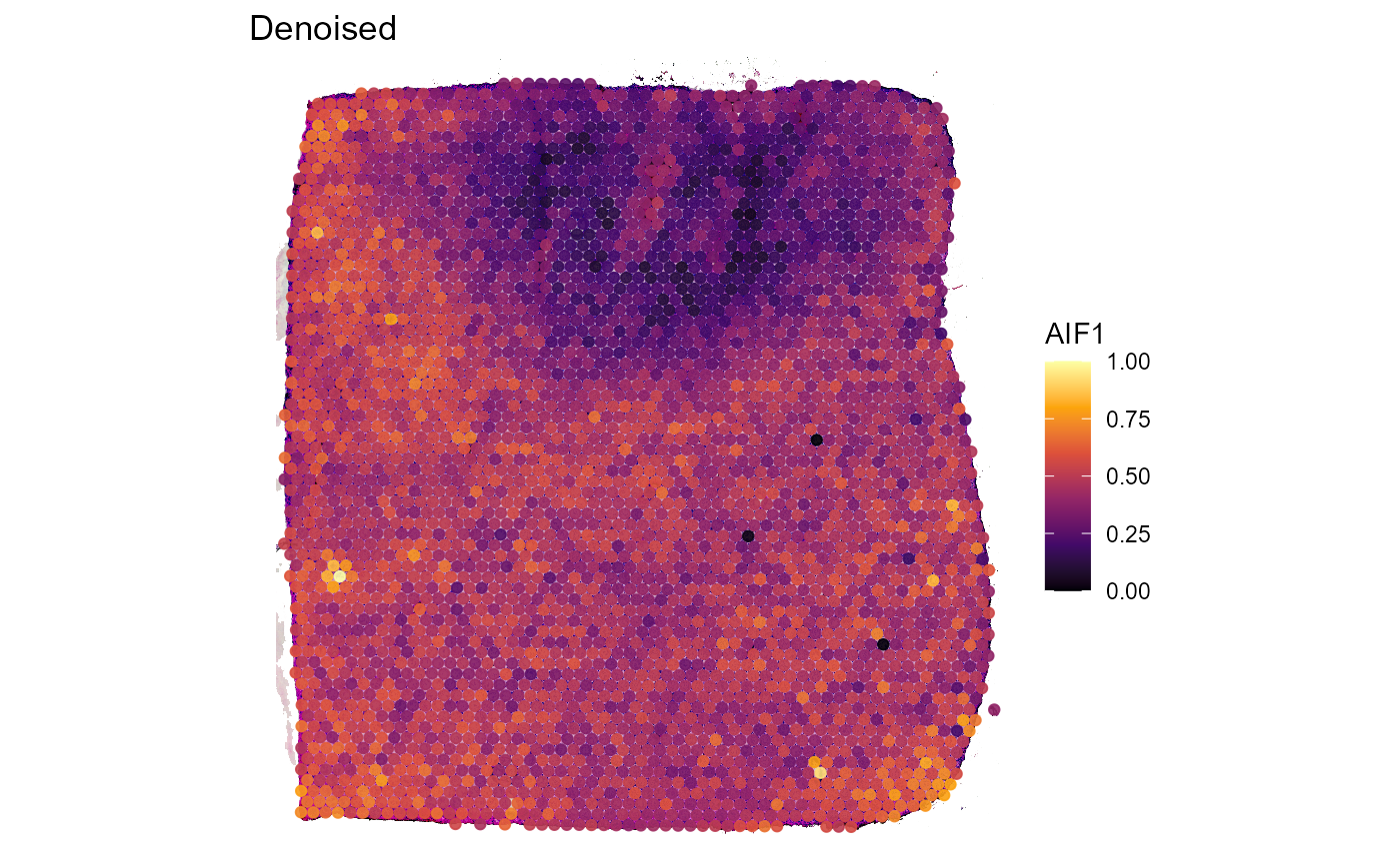
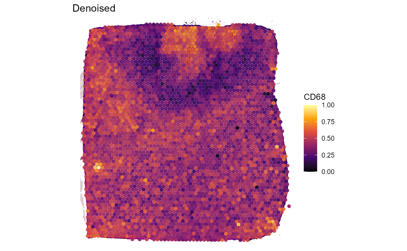
Figure 3.3 Denoised expression of genes AIF1 and CD68
The prominent changes of the coloring between surface plots from the
scaled expression matrix (Figure 3.2) and from the denoised one (Figure
3.3) results from the autoencoder network returning normally distributed
values while the majority of results from count normalization and
scaling are not normally distributed. To visualize differences between
the scaled and the denoised expression matrix you can either use
functions that visualize the distribution of numeric variables (such as
plotDensityplot(), plotViolinplot() etc.) in
combination with setActiveMatrix() as shown in Figure 3.4
or you can use the function plotAutoencoderResults() as
shown in Figure 3.5.
spata_obj <- setActiveMatrix(object = spata_obj, mtr_name = "scaled")

plotViolinplot(
  object = spata_obj,
  variables = example_genes,
  display_facets = FALSE
  ) +
  labs(title = "Scaled (not denoised)")

spata_obj <- setActiveMatrix(object = spata_obj, mtr_name = "denoised")

plotViolinplot(
  object = spata_obj,
  variables = example_genes,
  display_facets = FALSE
  ) +
  labs(title = "Denoised")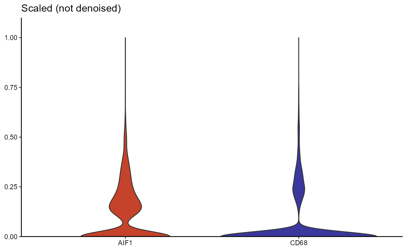
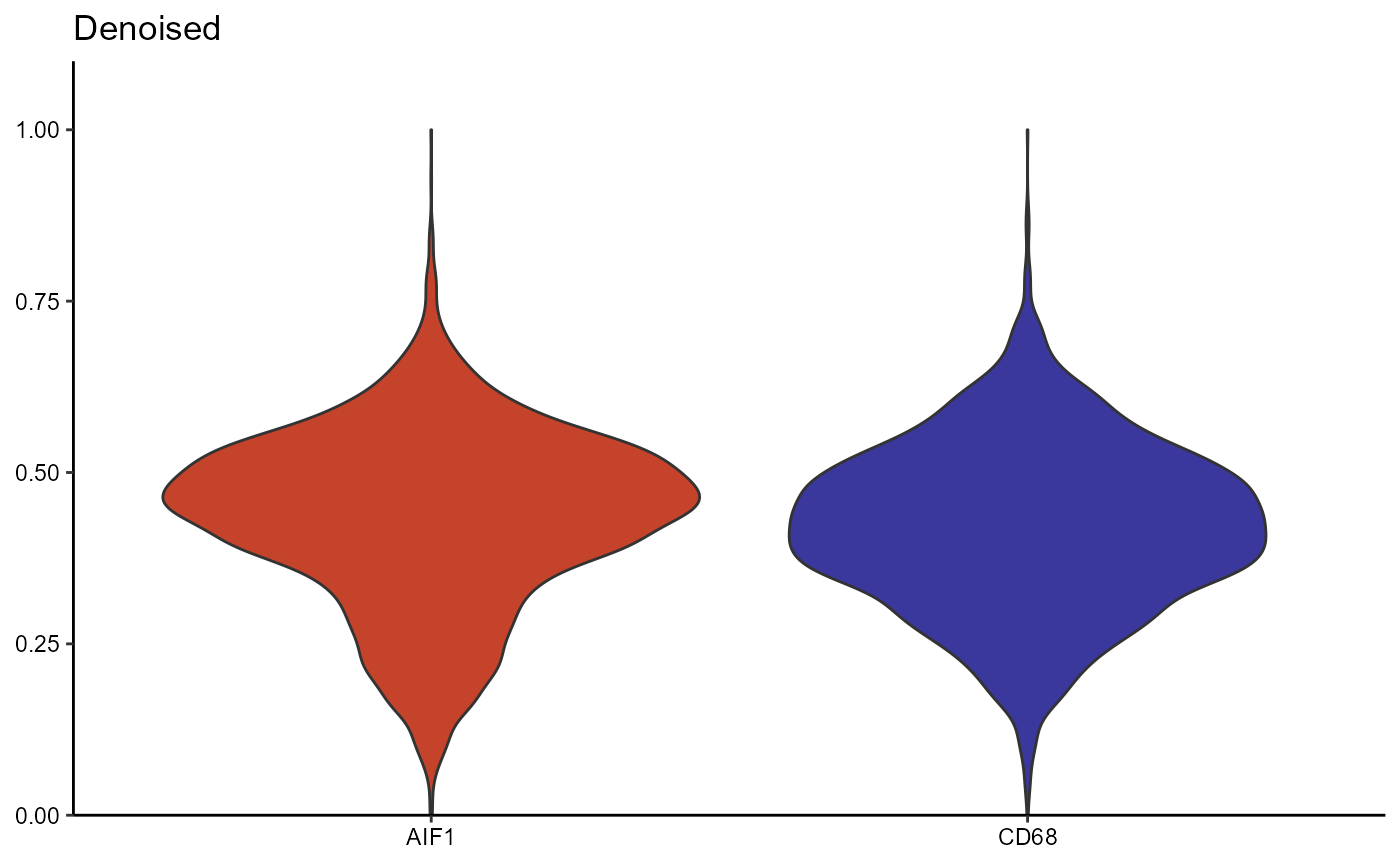
Figure 3.4 Differences in distribution between scaled and denoised expression (violinplot)
plotAutoencoderResults(
  object = spata_obj,
  genes = example_genes,
  pt_alpha = 0.4,
  pt_size = 1.25
  )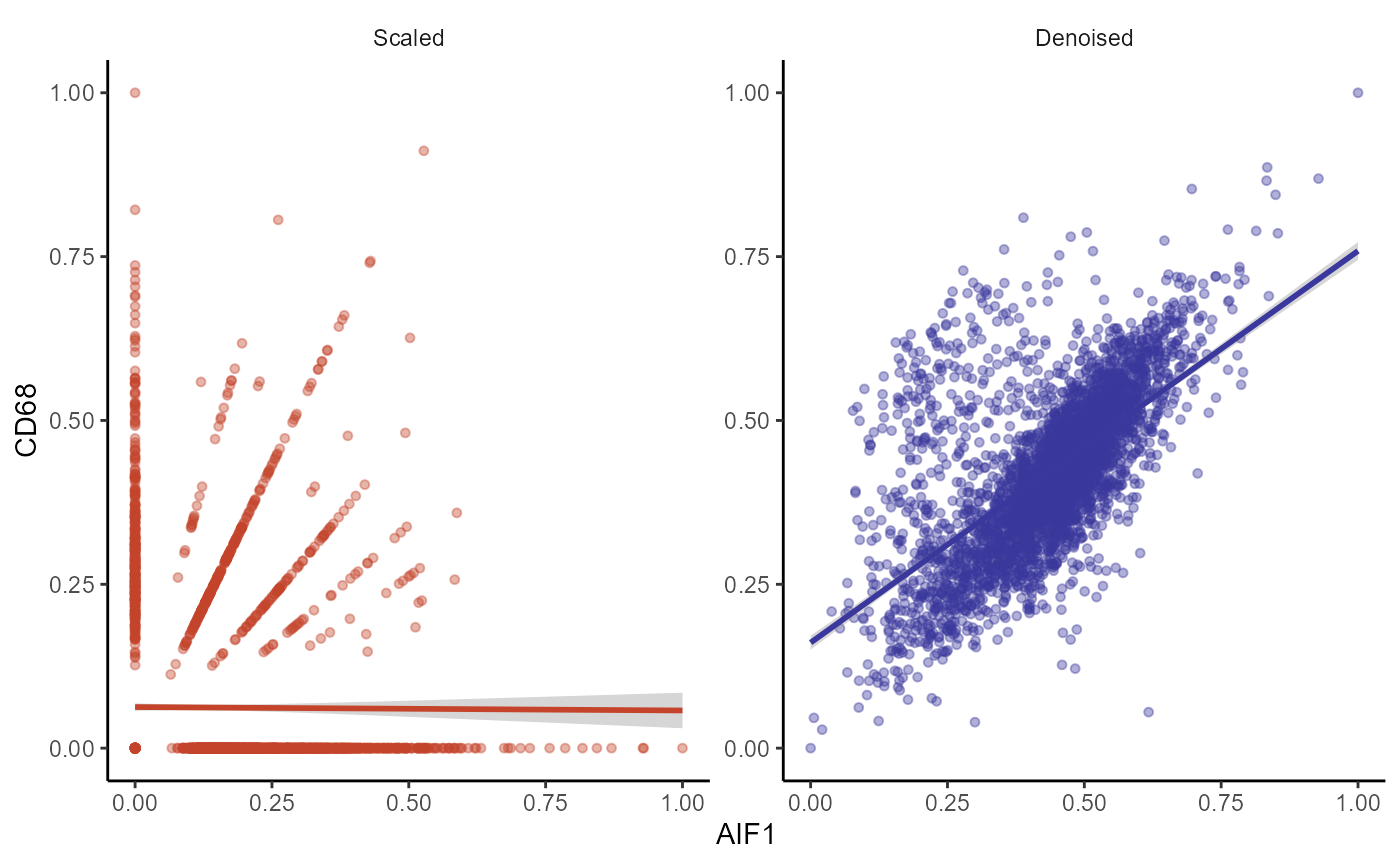
Figure 3.5 Differences in distribution between scaled and denoised expression (scatterplot)