Copy Number Variations (CNV)
spata-v2-cnv-analysis.Rmd2. Introduction
InferCNV is used to identify large-scale chromosomal copy number alterations in single cell RNA-Seq data including gains or deletions of chromosomes or large segments of such. Several publications have leveraged this technique. (Patel et al., 2014, Tirosh et al., 2016, Venteicher et al., 2017 )
Note: We are currently encountering problems with the function
infercnv:::plot_cnv(). It does not prevent the copy number
variation analysis. Sometimes, however, the heatmap is not plotted.
Checkout your R console for hints in how far the function did not work
properly. We are working on a solution for that. If you encounter
warnings raised from runCnvAnalysis() let us know.
# load package
library(tidyverse)
library(SPATA2)
library(SPATAData)

object_t269 <- downloadSpataObject(sample_name = "269_T")

# load histolgoy segmentations
data("spatial_segmentations")

object_t269 <-
  addFeatures(
    object = object_t269,
    feature_df = spatial_segmentations[["269_T"]],
    overwrite = TRUE
  )

# only histology
plotSurface(object, = object_t269, pt_alpha = 0)

# histological grouping
plotSurface(object = object_t269, color_by = "histology")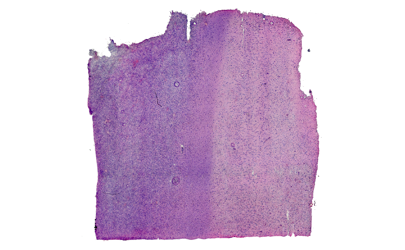
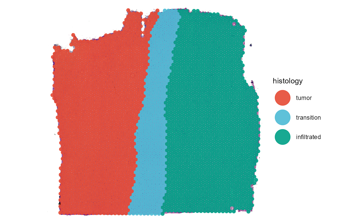
Fig.1 The example sample raw and colored by histological classification.
SPATA2 implements the package infercnv
published and maintained by Broadinstitute and allows to integrate this
technique in your workflow of analyzing spatial trancsriptomic data
derived from malignancies.
3. Running CNV-Analysis
As with all other functions prefixed with run*() the
function runCnvAnalysis() is a wrapper around all necessary
functions needed to conduct copy-number-variation-analysis. The results
needed for subsequent analysis steps are stored in the specified
spata2 object (slot: @cnv).
The infercnv-object is stored in the folder specified in the argument
directory_cnv_folder.
object_t269 <-
  runCnvAnalysis(
    object = object_t269,
    directory_cnv_folder = "data-gbm269/cnv-results", # example directory
    cnv_prefix = "Chr"
    )
If your desired set up deviates from the default you can reach any
function of the inferncnv pipeline by entering it’s name as
an argument and specify it’s input as a list of arguments with which you
want it to be called.
Copy number variation analysis requires reference data. This includes
a count matrix from healthy tissue, an annotation file as well as a
data.frame that contains information about the chromosome positions. We
provide reference data in the list SPATA2::cnv_ref.
names(cnv_ref)## [1] "annotation" "mtr" "regions"
summary(cnv_ref)## Length Class Mode
## annotation 1 data.frame list
## mtr 71067022 -none- numeric
## regions 4 data.frame listrunCnvAnalysis() defaults to the content of this list.
The documentation of runCnvAnalysis() contains a detailed
description of the requirements each reference input must meet in order
for the function to work.
4. CNV-Results
The results are stored in a list inside the spata2
object. This list can be obtained via getCnvResults().
cnv_results <- getCnvResults(object_t269)

names(cnv_results)
## [1] "prefix" "cnv_df" "cnv_mtr" "gene_pos_df" "regions_df"5. Visualization
5.1 Heatmap
The gains and losses of chromosomal segments can be displayed via
plotCnvHeatmap().
plotCnvHeatmap(object = object_t269)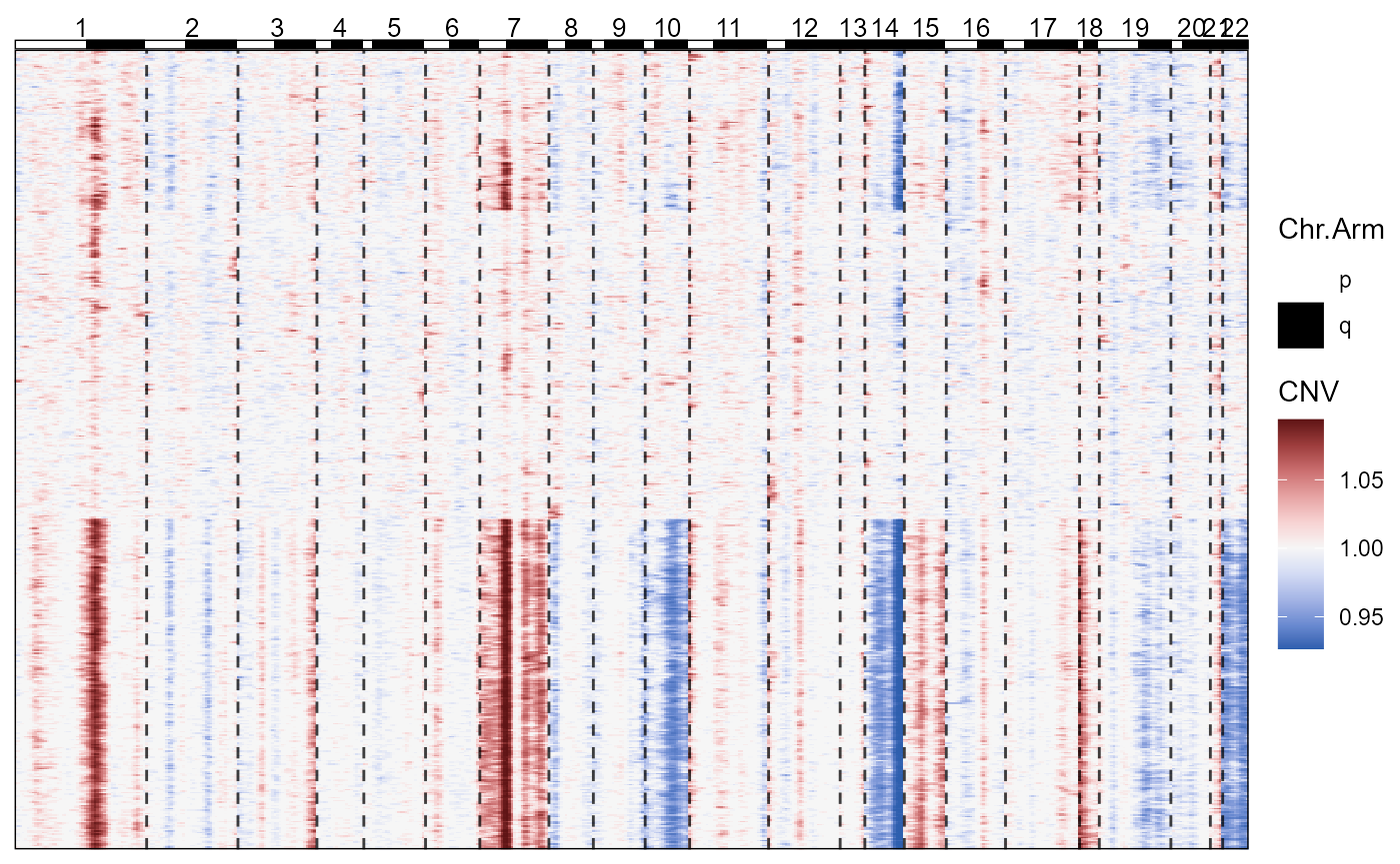
Fig.2 Basic CNV-Heatmap.
If you want to visualize the results across certain groups to
identify subclones make use of the across-argument.
plotCnvHeatmap(object = object_t269, across = "histology", clrp = "npg")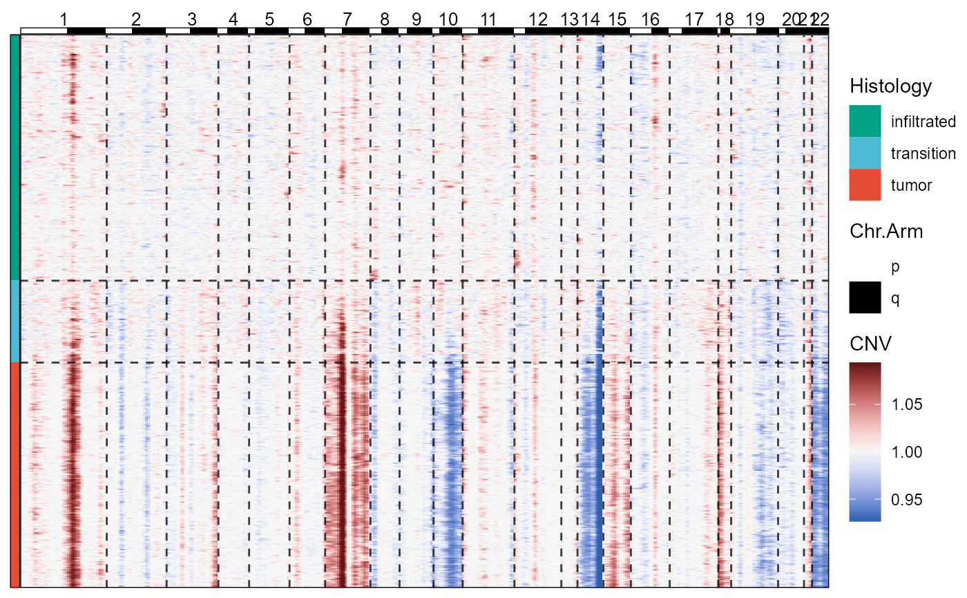
Fig.3 CNV-Heatmap with meta data displayes chromosomal alterations across histological classification.
5.2 Lineplot
An additional option to visualize the results provides
plotCnvLineplot().
plotCnvLineplot(
  object = object_t269,
  across = "histology",
  n_bins_bcsp = 1000,
  n_bins_genes = 1000,
  nrow = 3
)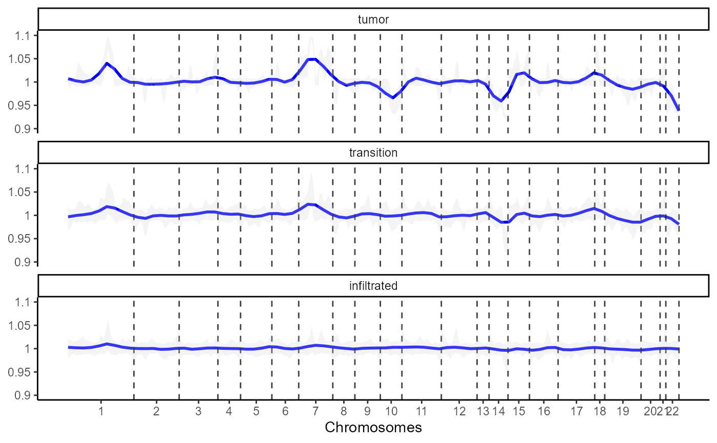
Fig.4 CNV-Lineplot displays chromosomal changes across histological classification.
5.3 Surface
The numeric values by which the copy number variations of each
chromosome are represented are immediately transferred to the
spata2 object’s feature data and are thus accessible for
all functions that work with numeric variables. The character string
specified in argument cnv_prefix combined with the
chromosomes number determines the name by which you can refer to these
feature variables.
# cnv feature names
getCnvFeatureNames(object = object_t269)
## [1] "Chr1" "Chr2" "Chr3" "Chr4" "Chr5" "Chr6" "Chr7" "Chr8" "Chr9"
## [10] "Chr10" "Chr11" "Chr12" "Chr13" "Chr14" "Chr15" "Chr16" "Chr17" "Chr18"
## [19] "Chr19" "Chr20" "Chr21" "Chr22"
# are part of all feature names
getFeatureNames(object = object_t269)
## numeric integer factor numeric
## "nCount_Spatial" "nFeature_Spatial" "seurat_clusters" "Chr0"
## numeric numeric numeric numeric
## "Chr1" "Chr10" "Chr11" "Chr12"
## numeric numeric numeric numeric
## "Chr13" "Chr14" "Chr15" "Chr16"
## numeric numeric numeric numeric
## "Chr17" "Chr18" "Chr19" "Chr2"
## numeric numeric numeric numeric
## "Chr20" "Chr21" "Chr22" "Chr23"
## numeric numeric numeric numeric
## "Chr3" "Chr4" "Chr5" "Chr6"
## numeric numeric numeric factor
## "Chr7" "Chr8" "Chr9" "histology"Use plotSurface() to visualize chromosomal alterations
directly on the histology.
plotSurface(
  object = object_t269,
  color_by = "Chr7",
  pt_clrsp = "Reds"
)

plotSurface(
  object = object_t269,
  color_by = "Chr10",
  pt_clrsp = "Oslo"
)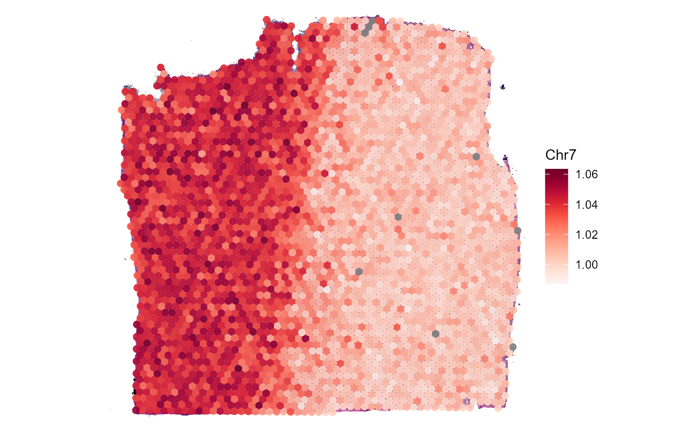
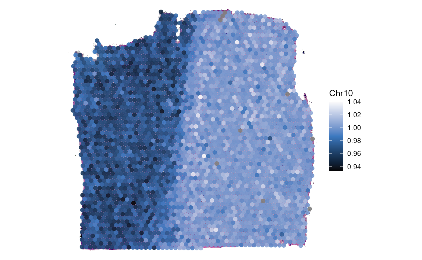
Fig.5 Surface plots display chromosomal alterations directory on the histology.
5.4 Gradients
As showcased in our corresponding vignette about spatial trajectories gradients of numeric variables can be displayed. Chromosomal alterations are numeric variables.
object_t269 <-
    setTrajectory(
      object = object_t269,
      trajectory = spatial_trajectories[["269_T"]][["horizontal_mid"]],
      overwrite = TRUE
    )

plotSpatialTrajectories(
  object = object_t269,
  ids = "horizontal_mid",
  color_by = "Chr7",
  pt_clrsp = "Reds 3"
)

plotSpatialTrajectories(
  object = object_t269,
  ids = "horizontal_mid",
  color_by = "Chr10",
  pt_clrsp = "Oslo"
)

plotTrajectoryLineplot(
  object = object_t269,
  id = "horizontal_mid",
  variables = "Chr7",
  line_color = "red"
)

plotTrajectoryLineplot(
  object = object_t269,
  id = "horizontal_mid",
  variables = "Chr10",
  line_color = "blue",
  x_nth = 4
)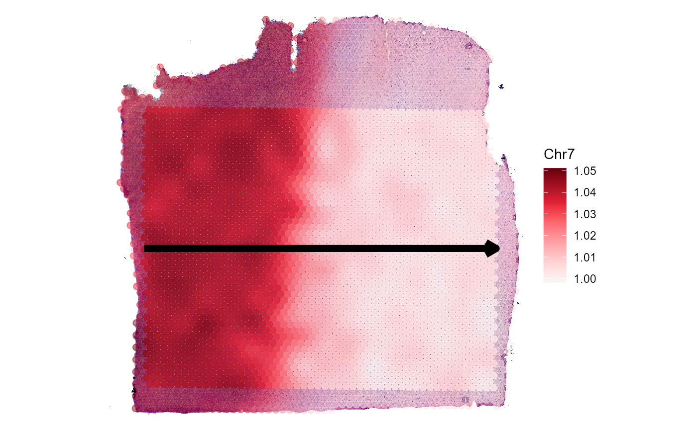
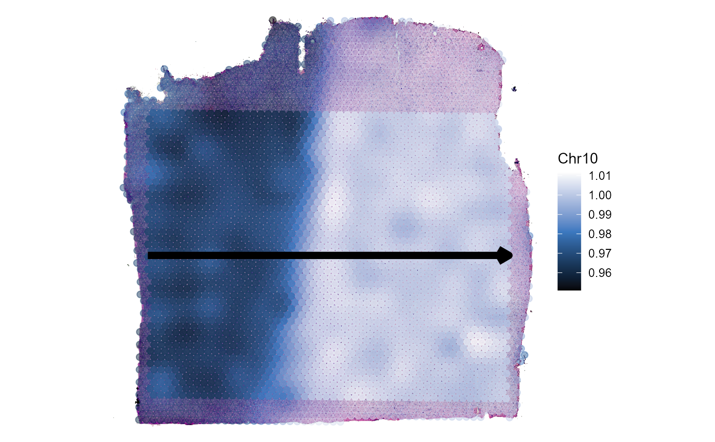
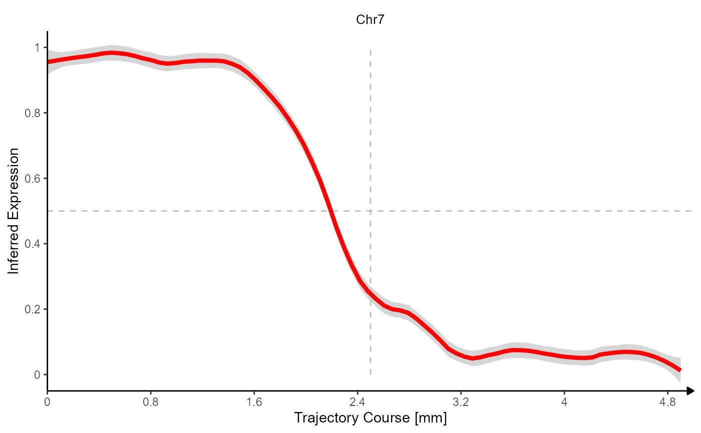
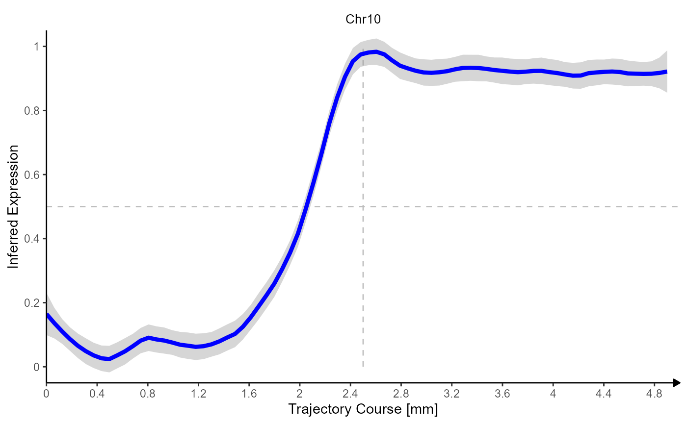
Fig.6 Gradients of Chromosomal alterations along a trajectory in space.
(Note that trajectory lineplots always rescale variables to 0-1 or to low-high.)