Miscellaneous plots

1. Prerequisites

None.

2. Introduction

This vignette gives examples of a variety of different plotting options SPATA2 offers.

object_t275 <- downloadSpataObject("275_T")

data("clustering")

object_t275 <- 
  addFeatures(
    object = object_t275, 
    feature_df = clustering$`275_T`, 
    overwrite = TRUE
  )

object_t275 <- setDefault(object_t275, pt_clrp = "jama")

plotSurface(object_t275, color_by = "bayes_space")

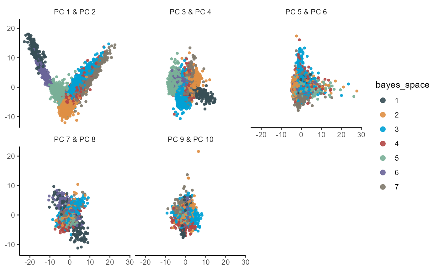
3. Dimensional reduction

Dimensional reduction in form of PCA, TSNE and UMAP can be plotted with the respective functions plotPca(), plotTSNE() and plotUmap().

plotPca(
  object = object_t275, 
  n_pcs = 10, 
  color_by = "bayes_space", 
  pt_size = 1
)

plotTsne(object_t275, color_by = "bayes_space", pt_size = 1)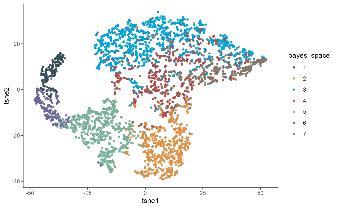

plotUmap(object_t275, color_by = "bayes_space", pt_size = 1)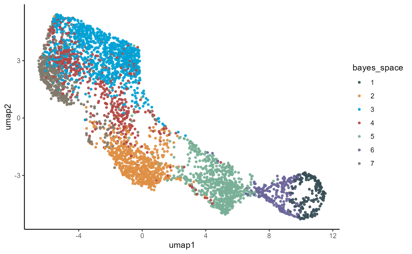

To plot multiple dimensional reduction plots with different variables color_by can be of length bigger than 1 as long as all variables are numeric.

4. Statistics

Statistic related plots can be plotted via plotBoxplot(), plotViolinplot(), plotRidgeplot(), plotDensityplot() and plotHistogram(). The first two allow for statistical tests.

object_t275 <- setDefault(object_t275, clrp = "Set3")

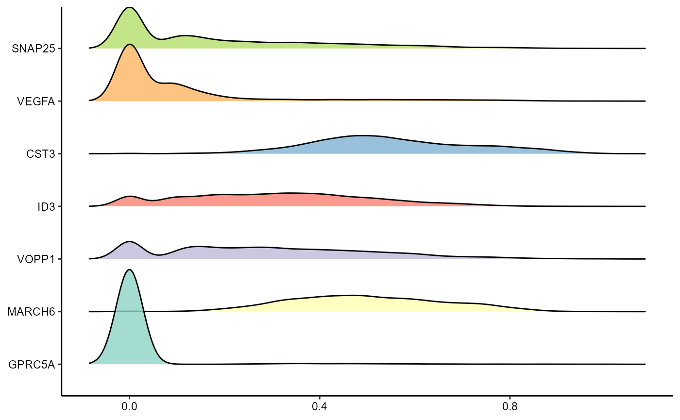
plotRidgeplot(
  object = object_t275, 
  variables = dea_genes
)

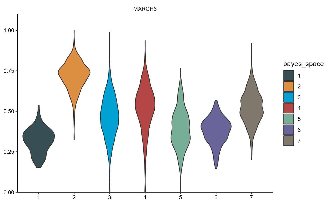
Use argument across if you want to do display value distribution across groups and perform statistical tests.

# show results 
dea_genes
##        1        2        3        4        5        6        7 
## "GPRC5A" "MARCH6"  "VOPP1"    "ID3"   "CST3"  "VEGFA" "SNAP25"

# plot results
plotViolinplot(
  object = object_t275, 
  across = "bayes_space",
  variables = dea_genes[2], 
  clrp = "jama"
)

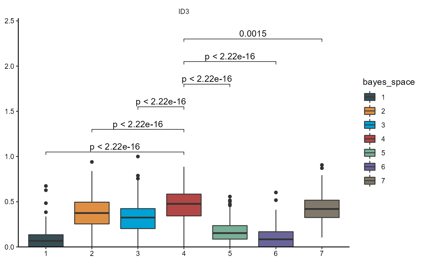
Statistical tests can be added to the plot via the arguments test_groupwise and test_pairwise.

plotBoxplot(
  object = object_t275, 
  variables = dea_genes[4],
  across = "bayes_space",
  test_pairwise = "t.test",
  step_increase = 0.25,
  ref_group = "4",
  clrp = "jama"
)

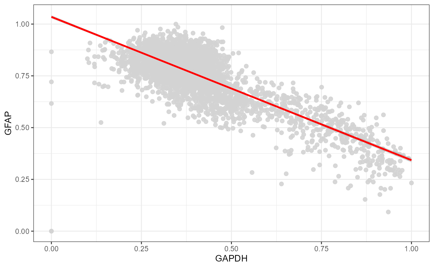
5. Scatterplots

plotScatterplot() includes multiple options to plot two numeric variables against each other.

plotScatterplot(
  object = object_t275, 
  variables = c("GAPDH", "GFAP"), 
  smooth = TRUE, 
  smooth_method = "lm"
)