Image Annotation Screening
spata-v2-image-annotation-screening.Rmd1. Requisites
Make sure to be familiar with the following vignettes:
- Image Annotations
- Spatial Segmentation vs. Image Annotations - Code & Concept
- Image Annotation Screening - Code & Concept
- Model Fitting in Spatial Transcriptomic Studies - Code & Concept
This one might help, too:
2. Introduction & overview
Many algorithms have been developed to identify genes in spatial transcriptomic studies that are expressed in a spatially meaningful manner. E.g. SPARKX, Trendseek, SpatialDE. Drawback of these algorithms is that they only detect genes of interest but rarely come with additional information that allow biological interpretation. Additionally, they always take the sample as a whole and do not allow the user to specify histological regions of interest that require further investigation regarding the impact they have on the rest of the sample. To address this, we have created Image annotations screening (IAS). In combination with our recently introduced image annotation system, IAS allows to screen for genes that feature interesting expression patterns in relation to histological structures or user defined regions as a function of distance to them.
This tutorial guides you through all of its main functions. For a more detailed explanation on how IAS works click here to be guided to the code and concept behind image annotation screening.
library(SPATA2)
library(SPATAData)
library(tidyverse)

object_t313 <- SPATAData::downloadSpataObject(sample_name = "313_T", file = NULL)

object_t313 <- setDefault(object_t313, pt_clrsp = "Reds 3", display_image = FALSE)
3. Setting up the algorithm
Image annotation screening requires four aspects must be specified.
- The image annotation that encircles the area of interest, using
argument
id.
- The image annotation that encircles the area of interest, using
argument
- The area surrounding the image annotation that is screened. This is
done with a combination of arguments
distance,binwidthandn_bins_circle.
- The area surrounding the image annotation that is screened. This is
done with a combination of arguments
- Further confinement of the area by angle, using argument
angle_span.
- Further confinement of the area by angle, using argument
- The resolution of the screening, using argument
n_bins_angle.
- The resolution of the screening, using argument
3.1 The image annotation of interest
At first, the area of interest must be captured within an image
annotation. This is done with createImageAnnotation(). The
sample that will be used in this tutorial is the same as the one that’s
used in the image annotation tutorial. Example image
annotations are provided in the list image_annotationsand
can be directly added using setImageAnnotation(). The image
annotation that is used throughout this vignette encircles a necrotic
area that is located in the center of the Glioblastoma. It carries the
ID necrotic_center.
# load example list
data("image_annotations")

# load example or create interactively with createImageAnnotations()
object_t313 <-
  setImageAnnotation(
    object = object_t313,
    img_ann = image_annotations[["313_T"]][["necrotic_center"]],
    overwrite = TRUE
  )

plotImageGgplot(object = object_t313)

plotImageAnnotations(object = object_t313, ids = "necrotic_center", expand = 0.2)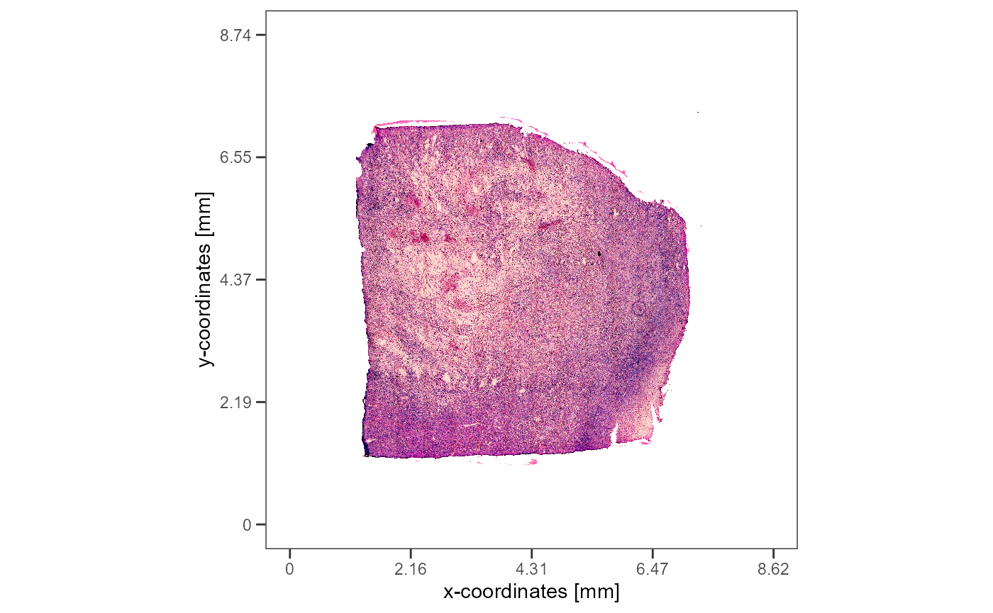
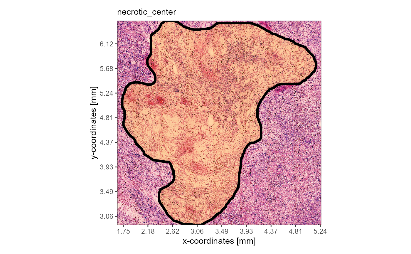
Fig.1 Glioblastoma T313 with it’s prominent necrosis region.
3.2 The area surrounding the image annotation
After deciding on the image annotation of interest with the argument
id, here id = 'necrotic_center', the area
around the image annotation that is included in the
screening process must be set up. To set up the area that is screened
two of the three arguments distance, binwidth
and n_bins_circle must be specified. The set up can be
checked and visualized with the function
plotSurfaceIAS().
bcsp_dist <- getCCD(object_t313, unit = "mm")

# show results
bcsp_dist
## 0.1 [mm]
plotSurfaceIAS(
  object = object_t313,
  id = "necrotic_center", # the ID of the image annotation of interest
  distance = "1mm",
  binwidth = bcsp_dist,
  pt_clrp = "milo", # use colorful panel to highlight the bins
  display_bins_angle = FALSE,
  ggpLayers = labs(subtitle = "a)")
)

plotSurfaceIAS(
  object = object_t313,
  id = "necrotic_center", # the ID of the image annotation of interest
  distance = "2.25mm", # covers the whole sample
  binwidth = bcsp_dist*2, # two layers of spots per bine
  display_bins_angle = FALSE,
  ggpLayers = labs(subtitle = "b)")
) 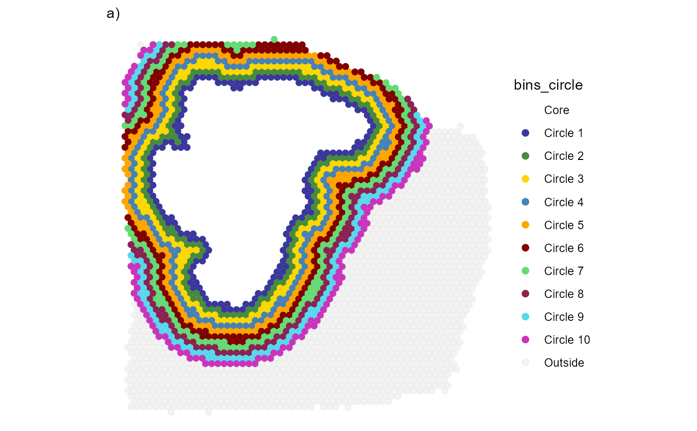

Fig.2 Visualize the area that is included in the screening process.
3.3 Further confining the area by angle
To further confine the screened area you can use
angle_span.
plotSurfaceIAS(
  object = object_t313,
  id = "necrotic_center", # the ID of the image annotation of interest
  distance = "2.25mm",
  binwidth = bcsp_dist,
  angle_span = c(45,225), # use angle_span to confine the area based on angle
  display_bins_angle = FALSE,
  ggpLayers = labs(subtitle = "a)")
)

plotSurfaceIAS(
  object = object_t313,
  id = "necrotic_center", # the ID of the image annotation of interest
  distance = "2.25mm",
  binwidth = bcsp_dist,
  angle_span = c(45, 225),
  display_bins_angle = FALSE,
  ggpLayers = labs(subtitle = "b)")
) 
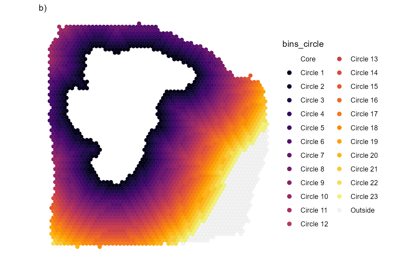
Fig.3 Confining the area by an angle span.
3.4 The resolution
Gene expression changes area inferred by binning the barcode-spots by
their distance to the area of interest and by aligning mean gene
expression of each bin. To increase the resolution, the barcode-spots
can be additionally binned by angle. Argument n_bins_angle
defaults to 1.
plotSurfaceIAS(
  object = object_t313,
  id = "necrotic_center",
  distance = "2.25mm",
  n_bins_angle = 1
  )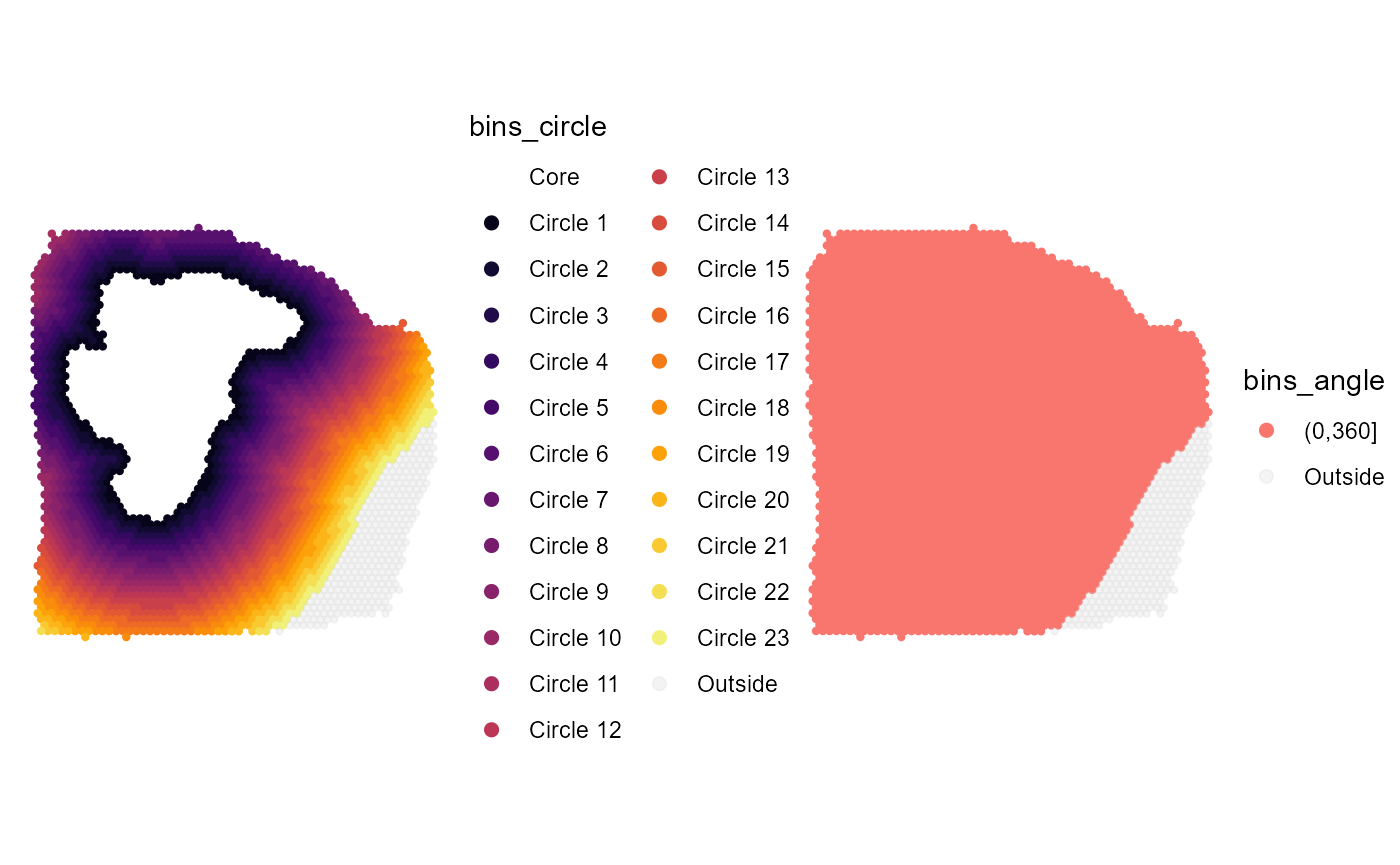
Fig.4 One angle bin.
By increasing n_bins_angle inferring gene expression
changes and the model fitting takes place within each angle-bin. The
final evaluation that tells whether a gene is expressed in an
e.g. descending way starting from the image annotation consists of a
summary of all gene-model-fits per angle bin.
plotSurfaceIAS(
  object = object_t313,
  id = "necrotic_center",
  distance = "2.25mm",
  n_bins_angle = 12
  )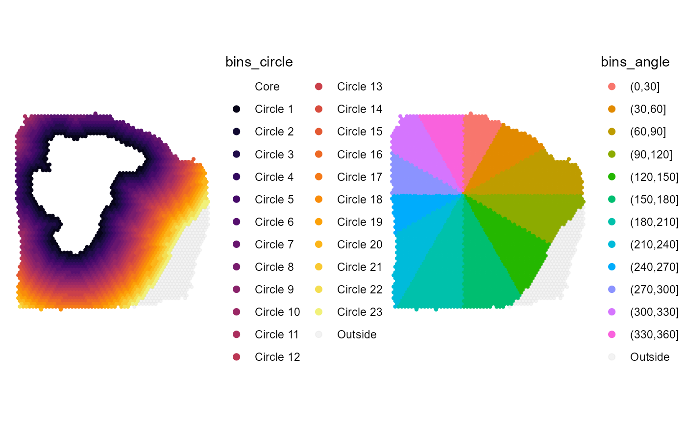
Fig.5 Twelve angle bins.
Increasing the resolution ensures that detected genes follow a certain trend everywhere around the image annotation which results in fewer false-positives but also in fewer true-positives. This is because genes might be excluded due to a bad evaluation in one angle-bin that might affect the overall evaluation in a way that it is discarded although within the remaining angle-bins the evaluation were good.
4. Running the algorithm
Once you’ve decided on the screening parameters, specify them within
the function imageAnnotationScreening() which runs the
algorithm. The parameter variables takes the numeric
variables that are included in the screening process. Usually it’s gene
names. Image annotation screening, however, is not restricted to genes
as virtually every numeric variable (e.g. nCount_Genes,
nCount_Features, gene sets, etc.) can be fitted to spatially
meaningful patterns, too. Therefore, the argument for the input is
simply called variables.
Here, we are using the genes that were already identified as spatially variable by SPARKX. The goal is to further analyze which of the genes are expressed in a spatial relation to the necrotic center. In particular, we want to find genes associated with necrosis using the descending models and genes repelled by necrosis using the ascending models.
# this is a wrapper around SPARK::sparkx()
object_t313 <- runSparkx(object = object_t313)

spark_df <- getSparkxGeneDf(object = object_t313, threshold_pval = 0.01)

# extract genes with a sparkx pvalue of 0.01 or lower
sparkx_genes <- spark_df[["genes"]]

# show results
spark_df

# show results (> 10 000 genes detected as spatially variable with a p-value of < 0.01)
str(sparkx_genes)
## # A tibble: 10,804 x 3
## genes combinedPval adjustedPval
## <chr> <dbl> <dbl>
## 1 B2M 7.11e-275 1.46e-269
## 2 SERF2 1.97e-261 2.02e-256
## 3 HLA-B 1.18e-247 8.07e-243
## 4 ACTB 3.33e-243 1.71e-238
## 5 MYL6 8.77e-241 3.60e-236
## 6 UBC 4.00e-238 1.37e-233
## 7 ATP5F1E 1.03e-231 3.02e-227
## 8 ACTG1 7.41e-229 1.91e-224
## 9 H3F3A 2.66e-227 6.07e-223
## 10 S100A11 2.29e-226 4.71e-222
## # i 10,794 more rows## chr [1:10804] "B2M" "SERF2" "HLA-B" "ACTB" "MYL6" "UBC" "ATP5F1E" "ACTG1" ...
# models that screen for genes that ...
models_of_interest <-
  c("linear_ascending", # ... increase gradually with the distance to the necrosis (repelled)
    "late_ascending", # ... increase logarithmically with the distance to necrosis (stronger repelled)
    "immediate_descending", # ... decrease logarithmically with the distance to necrosis (strongly associated)
    "linear_descending" # ... decrease gradually with the distance to necrosis (associated)
    )

n_bins_circle <- 20

showModels(
  input = n_bins_circle, # length of the model vector
  model_subset = models_of_interest
) +
  labs(x = "Circle Bins (Distance to Necrosis)")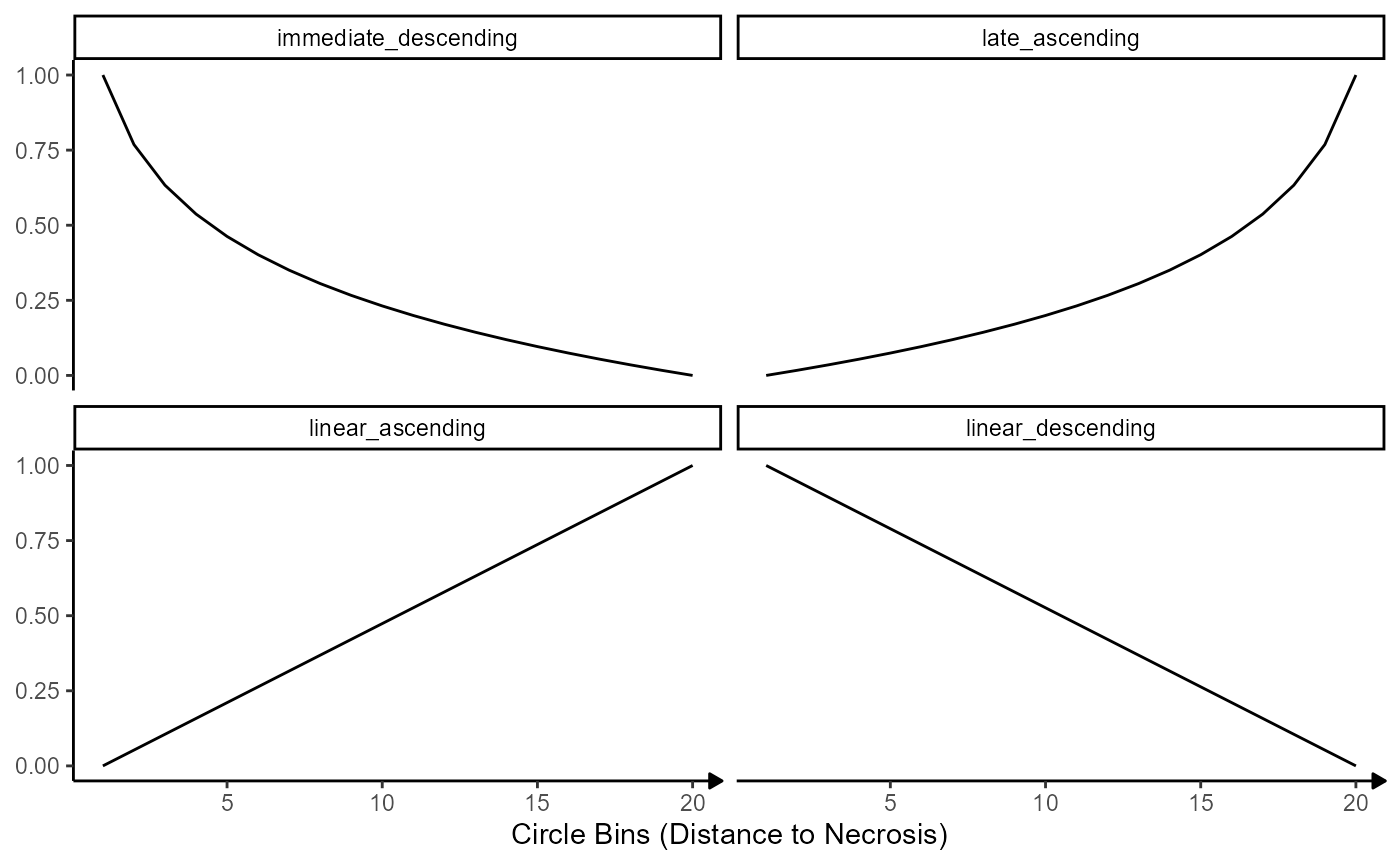
Fig.6 The models against which gene expression is fitted.
# run the algorithm and save the output in a new object
IAS_T313 <-
  imageAnnotationScreening(
    object = object_t313, # the spata object
    id = "necrotic_center", # the image annotation of interest
    variables = sparkx_genes, # the variables/genes to screen
    n_bins_circle = 20,
    distance = "2.25mm",
    model_subset = models_of_interest # the models against which all genes are fitted
  )
## 14:08:48 Specified `distance` = 2.25mm and `n_bins_circle` = 20. Calculated `binwidth` = 0.1125mm.Note: The output of
imageAnnotationScreening() is not saved in the
spata2 object but returned in a separate S4 object of class
ImageAnnotationScreening. Do not overwrite the
spata2 object by writing
object_t313 <- imageAnnotationScreening(object = object_t313, id = "necrotic_center", ...).
5. Results
5.1 Visualization
To get an overview of the screening as well as a first visualization
of the results use plotOverview. It sorts the genes by
their best model-fit and plots the evaluation score against the p-value
for every model.
plotOverview(
  object = IAS_T313,
  label_vars = 5,
  label_size = 3
  )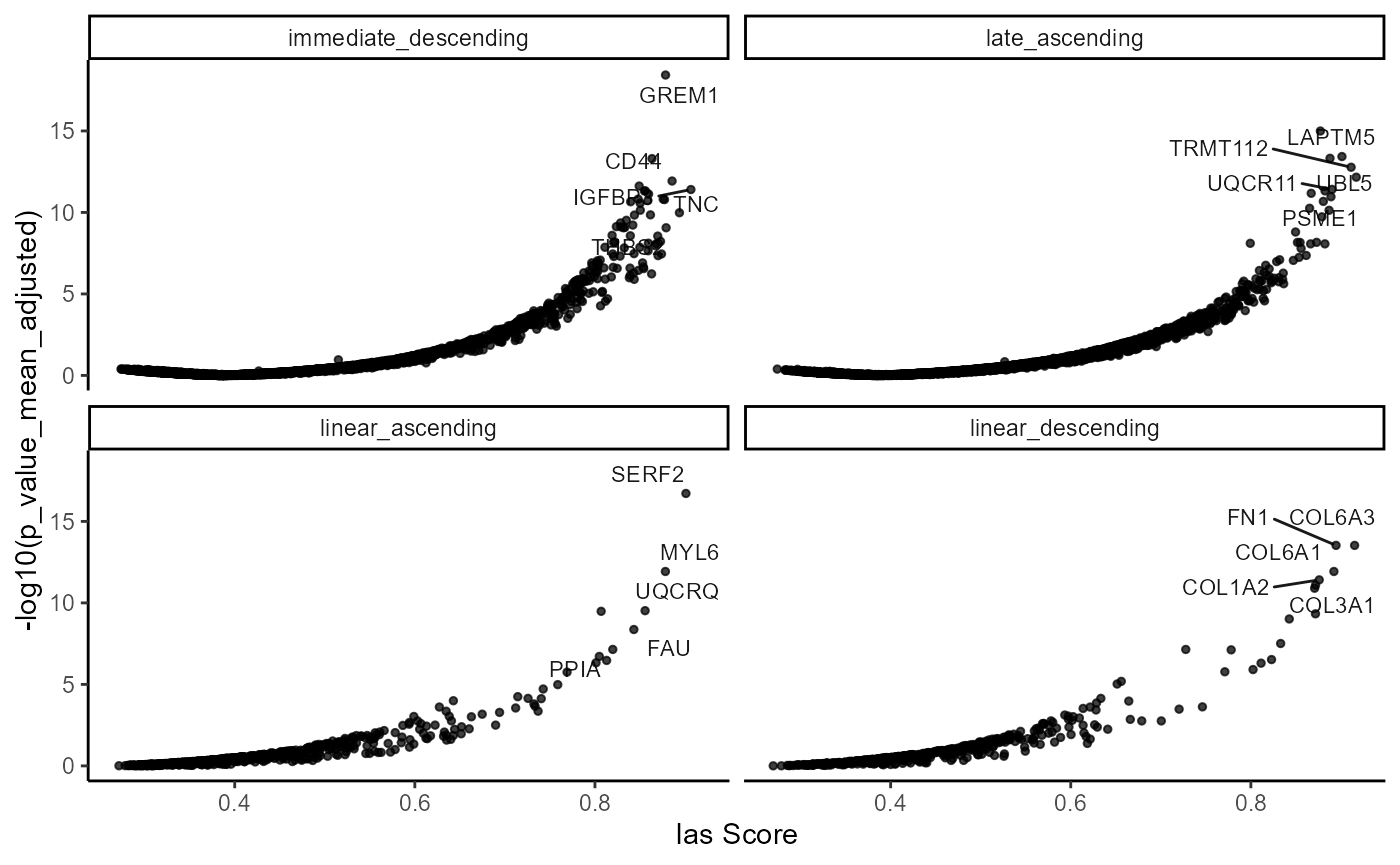
Fig.7 Visualize gene evaluation by model.
# using ten circle bins to visualize the concept
ias_layer_bins <-
  ggpLayerEncirclingIAS(
    object = object_t313,
    distance = "2.25mm",
    n_bins_circle = 10,
    id = "necrotic_center",
    line_size = 1
  )

# using only one circle bin to visualize the screening area
ias_layer_range <-
  ggpLayerEncirclingIAS(
    object = object_t313,
    distance = "2.25mm",
    n_bins_circle = 1,
    id = "necrotic_center",
    line_size = 1
  )

example_genes <-
  list(
    imm_desc = c("IGFBP3", "CD44"),
    lin_desc = c("FN1", "COL6A3"),
    lin_asc = c("SERF2", "MYL6"),
    late_asc = c("TRMT112", "LAPTM5")
    )

plotSurfaceComparison(
  object = object_t313,
  color_by = example_genes$imm_desc,
  nrow = 1
) +
  ias_layer_bins +
  labs(subtitle = "a) Immediate Descending")

plotSurfaceComparison(
  object = object_t313,
  color_by = example_genes$lin_desc,
  nrow = 1
) +
  ias_layer_range +
  labs(subtitle = "b) Linear descending")

plotSurfaceComparison(
  object = object_t313,
  color_by = example_genes$lin_asc,
  nrow = 1
) +
  ias_layer_range +
  labs(subtitle = "c) Linear ascending")

plotSurfaceComparison(
  object = object_t313,
  color_by = example_genes$late_asc,
  nrow = 1
) +
  ias_layer_range +
  labs(subtitle = "d) Late ascending")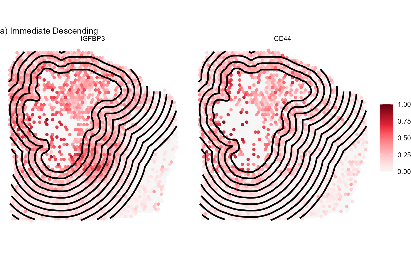
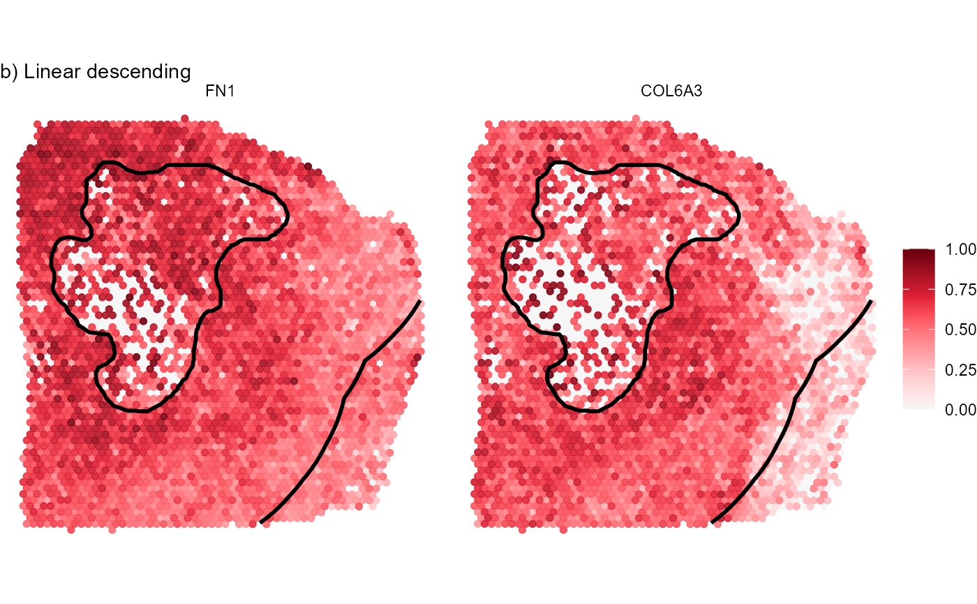
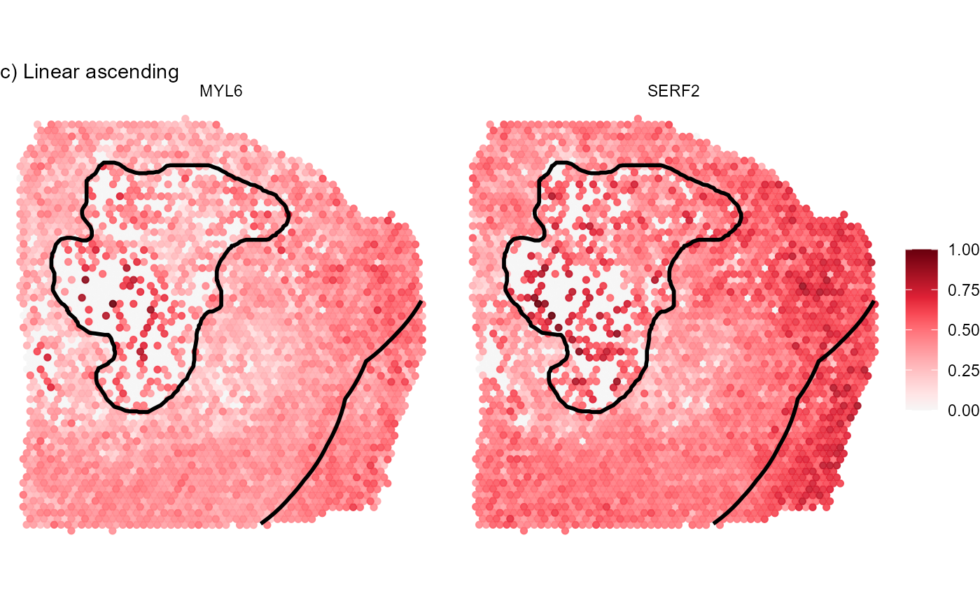
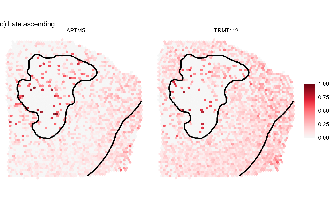
Fig.8 Visualize gene expression on the surface.
The inferred gene expression can be visualized with
plotIasLineplot().
genes_vec <- flatten_chr(example_genes)

plotIasLineplot(
  object = object_t313,
  id = "necrotic_center",
  distance = "2.25mm",
  n_bins_circle = 20,
  variables = genes_vec,
  include_area = FALSE,
  line_color = "red",
  display_border = TRUE,
  border_linesize = 0.75,
  border_linetype = "solid" # corresponds to the border of the image annotation
)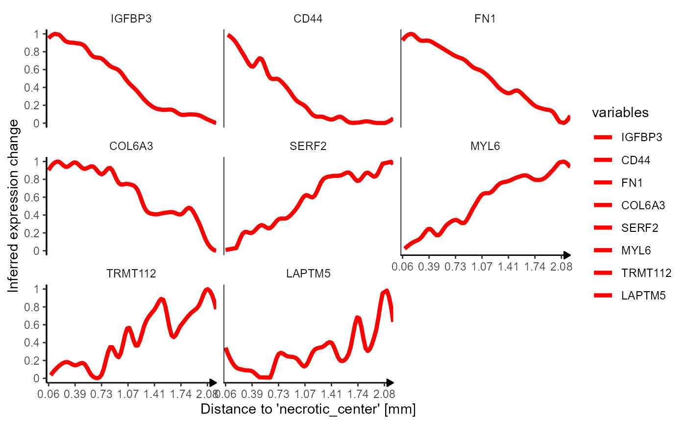
Fig.9 Lineplots used to visualize the inferred gene expression.
The function plotVolcano() makes use of the concept of
volcano plots as often used in DE-analyis to visualize the significance
as well as the log fold change of differentially expressed genes. Here
the left and the right side of the plot is used to display genes that
have inverse gene expression pattern.
plotVolcano(
  object = IAS_T313,
  left = "late_ascending",
  right = "immediate_descending",
  eval = "ias_score",
  pval = "p_value_mean_adjusted",
  threshold_eval = 0.75,
  threshold_pval = 0.05,
  label_vars = 5, # label the top 5 genes
  label_size = 3
  )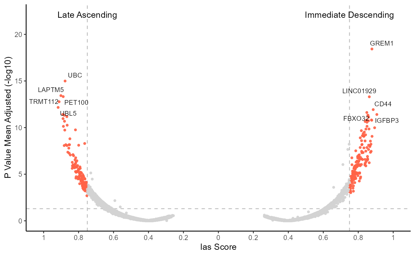
Fig.10 Visualize genes that have an inverse spatial expression pattern.
5.2 Extract results
Results can be extracted as data.frames with
getResultsDf() or as character vectors of variable names
with getResultsVec().
# complete results (left)
res_df_all <-
  getResultsDf(object = IAS_T313) %>%
  head(200)

# subset results (right)
res_df_best <-
  getResultsDf(
    object = IAS_T313,
    threshold_eval = 0.75,
    threshold_pval = 0.05,
    best_only = TRUE # only best model fit
  ) %>%
  head(200)
## # A tibble: 200 x 16
## # Groups: models [1]
## variables models ias_score n_bins_angle corr_mean corr_median corr_min
## <chr> <chr> <dbl> <int> <dbl> <dbl> <dbl>
## 1 IGFBP3 immediate_de~ 0.907 1 0.927 0.927 0.927
## 2 TNC immediate_de~ 0.894 1 0.904 0.904 0.904
## 3 CD44 immediate_de~ 0.886 1 0.934 0.934 0.934
## 4 THBS2 immediate_de~ 0.879 1 0.887 0.887 0.887
## 5 GREM1 immediate_de~ 0.878 1 0.979 0.979 0.979
## 6 P4HA2 immediate_de~ 0.877 1 0.917 0.917 0.917
## 7 ARL4C immediate_de~ 0.876 1 0.918 0.918 0.918
## 8 CTSK immediate_de~ 0.874 1 0.849 0.849 0.849
## 9 MMP2 immediate_de~ 0.873 1 0.869 0.869 0.869
## 10 LOXL2 immediate_de~ 0.870 1 0.846 0.846 0.846
## # i 190 more rows
## # i 9 more variables: corr_max <dbl>, corr_sd <dbl>, raoc_mean <dbl>,
## # p_value_mean <dbl>, p_value_median <dbl>, p_value_combined <dbl>,
## # p_value_mean_adjusted <dbl>, p_value_median_adjusted <dbl>,
## # p_value_combined_adjusted <dbl>## # A tibble: 200 x 16
## # Groups: models [2]
## variables models ias_score n_bins_angle corr_mean corr_median corr_min
## <chr> <chr> <dbl> <int> <dbl> <dbl> <dbl>
## 1 IGFBP3 immediate_de~ 0.907 1 0.927 0.927 0.927
## 2 TNC immediate_de~ 0.894 1 0.904 0.904 0.904
## 3 CD44 immediate_de~ 0.886 1 0.934 0.934 0.934
## 4 THBS2 immediate_de~ 0.879 1 0.887 0.887 0.887
## 5 GREM1 immediate_de~ 0.878 1 0.979 0.979 0.979
## 6 P4HA2 immediate_de~ 0.877 1 0.917 0.917 0.917
## 7 ARL4C immediate_de~ 0.876 1 0.918 0.918 0.918
## 8 CTSK immediate_de~ 0.874 1 0.849 0.849 0.849
## 9 MMP2 immediate_de~ 0.873 1 0.869 0.869 0.869
## 10 LOXL2 immediate_de~ 0.870 1 0.846 0.846 0.846
## # i 190 more rows
## # i 9 more variables: corr_max <dbl>, corr_sd <dbl>, raoc_mean <dbl>,
## # p_value_mean <dbl>, p_value_median <dbl>, p_value_combined <dbl>,
## # p_value_mean_adjusted <dbl>, p_value_median_adjusted <dbl>,
## # p_value_combined_adjusted <dbl>
imm_desc_genes <-
  getResultsVec(
    object = IAS_T313,
    model_subset = "immediate_descending",
    threshold_eval = 0.75,
    threshold_pval = 0.05
  ) %>%
  head(8) # keep top 8

#show results
imm_desc_genes
## immediate_descending immediate_descending immediate_descending
## "IGFBP3" "TNC" "CD44"
## immediate_descending immediate_descending immediate_descending
## "THBS2" "GREM1" "P4HA2"
## immediate_descending immediate_descending
## "ARL4C" "CTSK"
# plot results
plotSurfaceComparison(
  object = object_t313,
  color_by = imm_desc_genes,
  nrow = 2
) +
  ias_layer_range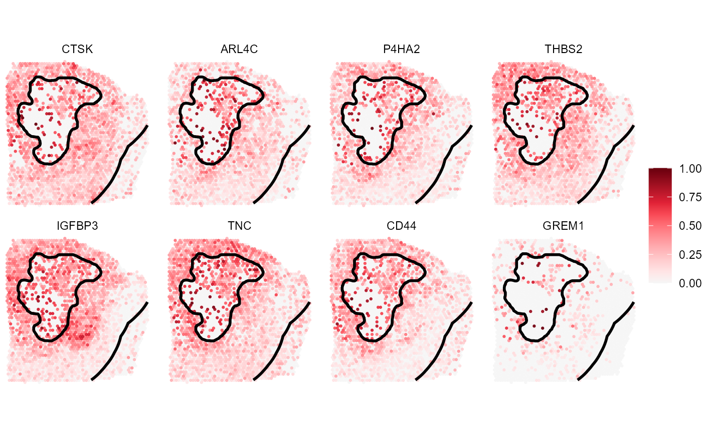
Fig.11 Top 8 genes that were identified as closely associated with necrosis.
late_asc_genes <-
  getResultsVec(
    object = IAS_T313,
    model_subset = "late_ascending",
    threshold_eval = 0.75,
    threshold_pval = 0.05
  ) %>%
  head(8) # keep top 8

#show results
late_asc_genes
## late_ascending late_ascending late_ascending late_ascending late_ascending
## "UBL5" "TRMT112" "LAPTM5" "UQCR11" "PSME1"
## late_ascending late_ascending late_ascending
## "PET100" "C12orf57" "TNFRSF12A"
# plot results
plotSurfaceComparison(
  object = object_t313,
  color_by = late_asc_genes,
  nrow = 2
) +
  ias_layer_range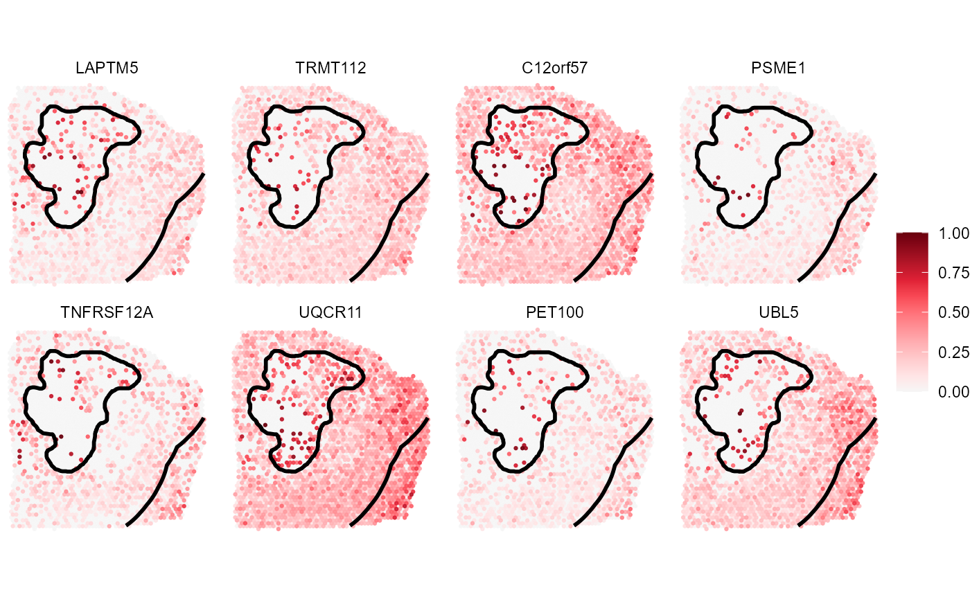
Fig.12 Top 8 genes that were identified as repelled with necrosis.
6. The S4 ImageAnnotationScreening class
Image annotation screening results are stored in an S4 object of
class ImageAnnotationScreening. Use
?ImageAnnotationScreening to read the description. Note
that ImageAnnotationScreening is the class name.
imageAnnotationScreening() is the function that runs
the algorithm.
class(IAS_T313)## [1] "ImageAnnotationScreening"
## attr(,"package")
## [1] "SPATA2"
slotNames(IAS_T313)## [1] "angle_span" "binwidth" "coords" "distance"
## [5] "img_annotation" "info" "method_padj" "models"
## [9] "n_bins_angle" "n_bins_circle" "results_primary" "results"
## [13] "sample" "summarize_with" "bcsp_exclude"