Spatial Annotation Screening

1. Introduction

This vignette exemplifies how to use Spatial Annotation Screening in SPATA2. It builds on the spatial annotations created in the vignette on creating spatial annotations.

library(SPATA2)
library(tidyverse)

# load SPATA2 inbuilt data and process
object_t313 <- loadExampleObject("UKF313T", process = TRUE, meta = TRUE)

necrotic_ids <- c("necrotic_area", "necrotic_edge", "necrotic_edge2")

plotSpatialAnnotations(object_t313, ids = necrotic_ids, nrow = 1)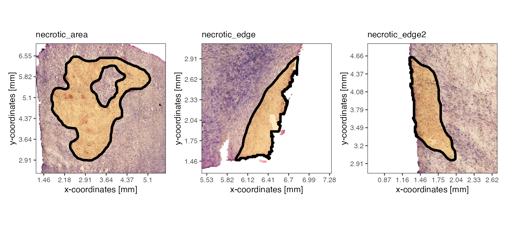

Spatial Annotation Screening (SAS) pursues the hypothesis that specific genes - or other numeric features for that matter - display non-random expression patterns in relation to spatial reference features, such as spatial annotations. SAS utilizes these reference features to incorporate the integration of potential biological forces in the identification of spatially variable genes, such as the presence of necrosis within a tumor. This allows for a supervised, hypothesis-driven screening for spatial patterns, which, unlike differential expression analysis (DEA), acknowledges the continuous nature of gene expression and avoids the limitations of group-based testing.

2. Running the algorithm

The algorithm is wrapped up in the function spatialAnnotationScreening(). Note that parameters core and distance are essential for the outcome. Make sure to align either input to your questioning. See the vignette on using spatial annotations for more information.

# prefiltering genes for spatial variability with SPARKX is recommended
object_t313 <- runSPARKX(object_t313)

sparkx_genes <- getSparkxGenes(object_t313, threshold_pval = 0.05)

sas_out <- 
  spatialAnnotationScreening(
    object = object_t313, 
    ids = necrotic_ids, 
    variables = sparkx_genes, 
    core = FALSE, # do not include the core of the annotations
    distance = "dte" # distance to edge 
  )

The output of spatialAnnotationScreening() is an S4 object of class SpatialAnnotationScreening which contains the set up as well as the results from the algorithm.

# an S4 object that contains the results 
class(sas_out)

## [1] "SpatialAnnotationScreening"
## attr(,"package")
## [1] "SPATA2"

slotNames(sas_out)

## [1] "annotations" "coordinates" "models"      "qc"          "results"    
## [6] "sample"      "set_up"

# prepare plotting 
screening_dir_layer <- ggpLayerScreeningDirectionSAS(object_t313, ids = necrotic_ids, line_size = 0.5)
sas_areas <- color_vector(clrp = "npg", names = c("core", "environment", "periphery"))

# left plot
# use information within the SAS output to recreate the set up 
plotSurface(sas_out, color_by = "rel_loc", clrp_adjust = sas_areas) +
  screening_dir_layer

# right plot
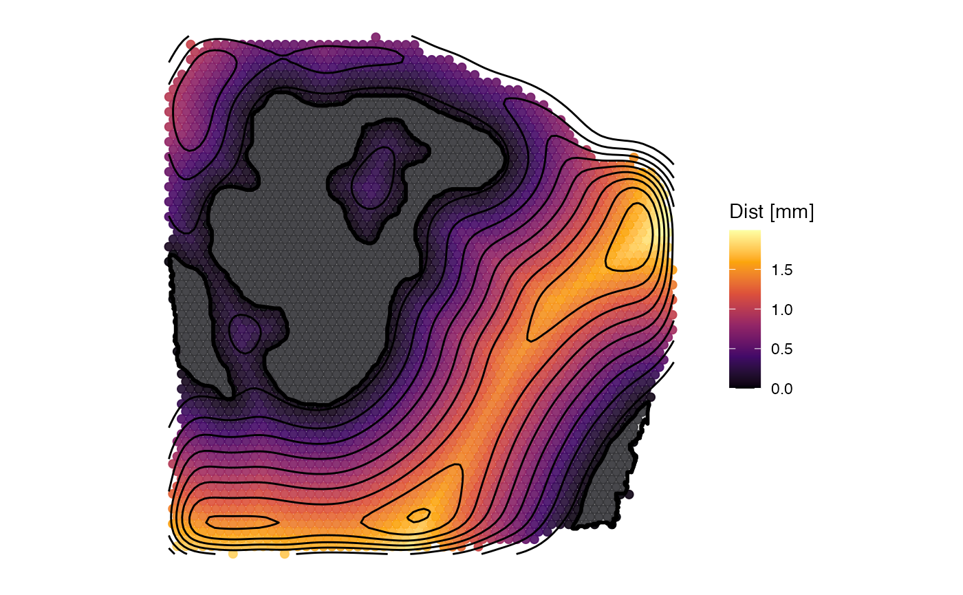
plotSurface(sas_out, color_by = "dist", fill = alpha("lightgrey", 0.25)) +
  labs(color = "Dist [mm]") + 
  screening_dir_layer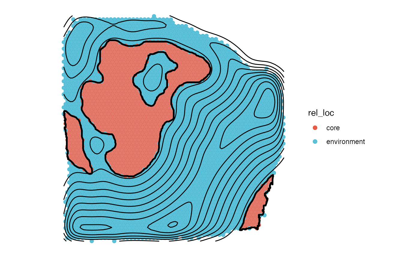

3. Extracting results

Results are stored in slot @results.

Slot @results$significance contains a data.frame with one row for each screened variable which provides information regarding the degree of randomness the inferred pattern contains as quantified by the total variation (tot_var). The p-value gives the probability to obtain such a total variation under complete randomness and indicates the degree of significance. Column fdr contains the adjusted p-value according to the False Discovery Rate.

Slot @results$model_fits contains the model fitting results. It is a data.frame where each row corresponds to a variable ~ model pair. The columns mae (mean absolute error) and rmse (root mean squared error) indicate the quality of the fit. The lower the value the better.

You can easily subset the results with dplyr verbs.

# e.g. filter output for gradients with a p-value less than 0.05
filter(sas_out@results$significance, p_value < 0.05)  

## # A tibble: 560 × 6
##    variables  rel_var tot_var p_value norm_var    fdr
##    <chr>        <dbl>   <dbl>   <dbl>    <dbl>  <dbl>
##  1 A2M          0.112    2.34  0.0091   0.117  0.0559
##  2 AC245595.1   1        2.33  0.0083   0.117  0.0513
##  3 ACTA2        0.516    2.13  0.0026   0.107  0.0235
##  4 ACTB         0.886    1.69  0        0.0846 0     
##  5 ACTG1       -0.569    1.82  0        0.0911 0     
##  6 ADAM12       0.361    2.50  0.0185   0.125  0.0852
##  7 ADD1        -0.426    2.32  0.0074   0.116  0.0474
##  8 ADM         -0.959    1.80  0        0.0898 0     
##  9 ADRM1        0.915    2.69  0.0361   0.135  0.125 
## 10 AKR1B1       1        2.26  0.0059   0.113  0.0418
## # ℹ 550 more rows

# e.g. filter model fits for best fit by variable
group_by(sas_out@results$model_fits, variables) %>% 
  slice_min(rmse, n = 1)

## # A tibble: 265 × 4
## # Groups:   variables [265]
##    variables models                mae   rmse
##    <chr>     <chr>               <dbl>  <dbl>
##  1 ACTA2     ascending_linear   0.236  0.266 
##  2 ACTB      ascending_linear   0.230  0.263 
##  3 ACTG1     peak_gradual       0.301  0.388 
##  4 ADD1      peak_gradual       0.290  0.353 
##  5 ADM       descending_gradual 0.0725 0.0970
##  6 AKR1B1    ascending_linear   0.153  0.206 
##  7 ANAPC11   ascending_linear   0.0976 0.123 
##  8 ANGPTL4   descending_linear  0.130  0.162 
##  9 APOC1     ascending_linear   0.102  0.131 
## 10 APOE      ascending_gradual  0.114  0.141 
## # ℹ 255 more rows

Alternatively, you can use getSgsResultsDf() and getSgsResultsVec() which are convenient wrappers around conditions with which to subset the results.

# the default: 
getSgsResultsDf(sas_out, pval = "fdr", threshold_pval = 0.05, eval = "mae", threshold_eval = 0.2)

## # A tibble: 207 × 9
## # Groups:   models [6]
##    variables models          mae   rmse rel_var tot_var p_value norm_var     fdr
##    <chr>     <chr>         <dbl>  <dbl>   <dbl>   <dbl>   <dbl>    <dbl>   <dbl>
##  1 CD74      ascending_l… 0.0550 0.0671   0.856    1.31  0        0.0655 0      
##  2 C1QB      ascending_l… 0.0570 0.0758   0.976    1.49  0        0.0743 0      
##  3 P4HA2     descending_… 0.0611 0.0782  -0.822    1.57  0        0.0783 0      
##  4 PSME2     ascending_l… 0.0627 0.0826   0.783    2.22  0.0041   0.111  0.0313 
##  5 FN1       descending_… 0.0653 0.0822  -0.910    1.77  0        0.0884 0      
##  6 NDUFA13   ascending_l… 0.0691 0.0883   1        1.77  0        0.0883 0      
##  7 THBS2     descending_… 0.0702 0.0919  -0.780    1.53  0        0.0763 0      
##  8 MFAP2     ascending_l… 0.0713 0.0853   0.994    1.30  0        0.0648 0      
##  9 ADM       descending_… 0.0725 0.0970  -0.959    1.80  0        0.0898 0      
## 10 IFITM3    ascending_l… 0.0727 0.105    0.720    1.92  0.0004   0.0962 0.00555
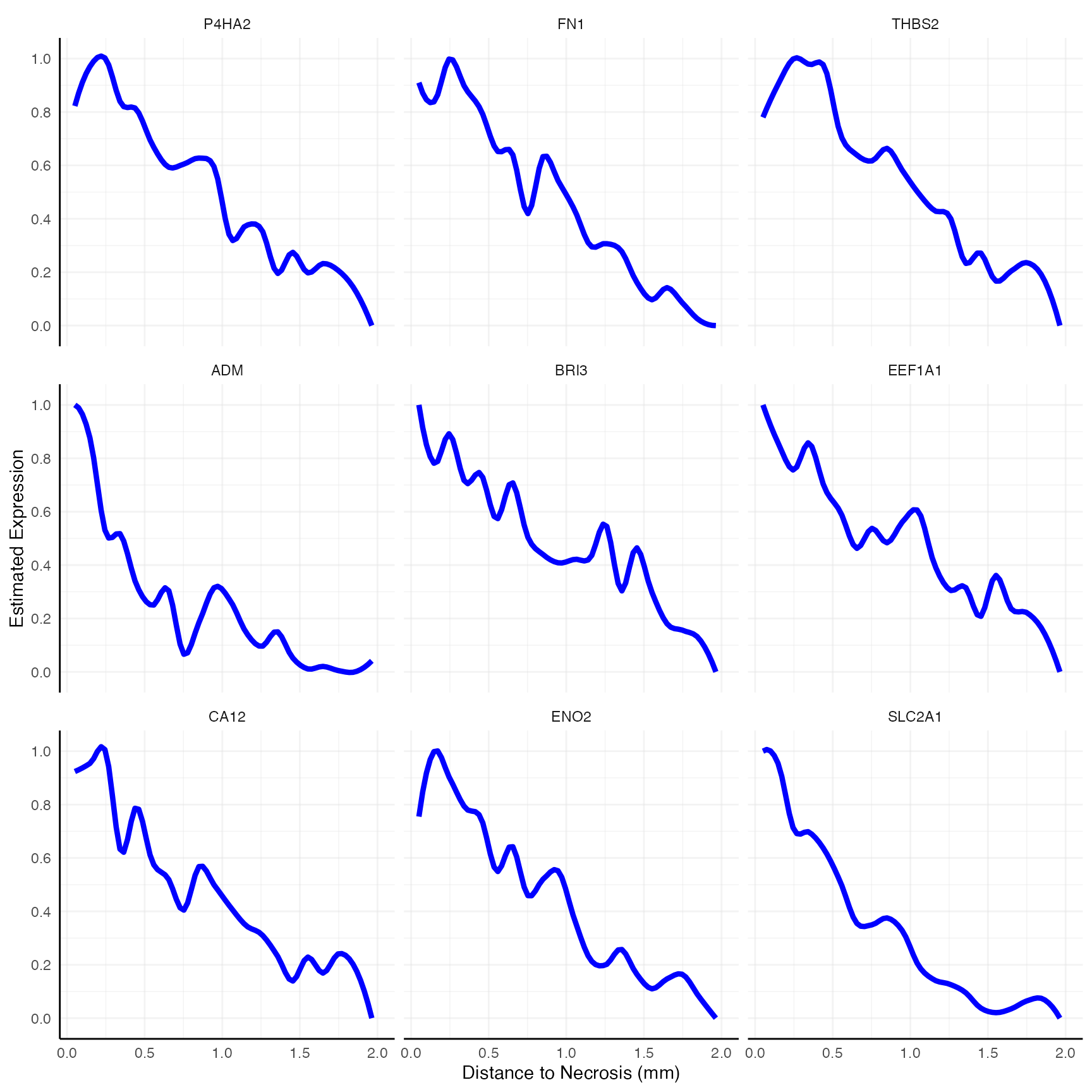
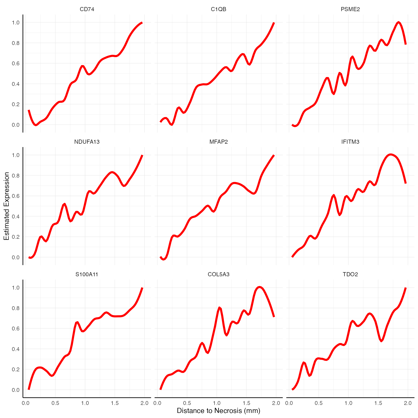
## # ℹ 197 more rows

You can filter the results for significant variables below a certain threshold for specific models to obtain genes of potential interest. For instance, to obtain genes that feature a non random, descending gradient with increasing distance to necrosis - associated with necrosis - use the following:

# (pval = "fdr", threshold_pval = 0.05)
desc_genes <- getSgsResultsVec(sas_out, model_subset = "descending")

length(desc_genes)

## [1] 63

head(desc_genes, 9)

## [1] "P4HA2"  "FN1"    "THBS2"  "ADM"    "BRI3"   "EEF1A1" "CA12"   "ENO2"  
## [9] "SLC2A1"

desc_genes_sub <- desc_genes[1:9]

# left plot
plotSurfaceComparison(
  object = object_t313, 
  color_by = desc_genes_sub,
  normalize = T, 
  outline = T, 
  pt_clrsp = "BuPu"
  ) + 
  ggpLayerSpatAnnOutline(object_t313, ids = necrotic_ids, fill = "grey", incl_edge = T)

# right plot
plotSasLineplot(
  object = object_t313, 
  variables = desc_genes_sub,
  ids = necrotic_ids, 
  line_color = "blue"
  ) + 
  labs(x = "Distance to Necrosis (mm)")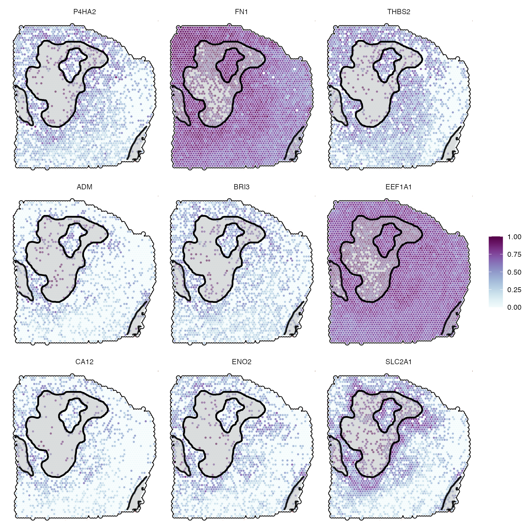

Alternatively, you can extract those with an opposite gradient - ascending ones - which correspond to genes rather repelled by necrosis.

# (pval = "fdr", threshold_pval = 0.05)
asc_genes <- getSgsResultsVec(sas_out, model_subset = "ascending")

length(asc_genes)

## [1] 176

head(asc_genes, 9)

## [1] "CD74"    "C1QB"    "PSME2"   "NDUFA13" "MFAP2"   "IFITM3"  "S100A11"
## [8] "COL5A3"  "TDO2"

asc_genes_sub <- asc_genes[1:9]

# show genes
asc_genes_sub

## [1] "CD74"    "C1QB"    "PSME2"   "NDUFA13" "MFAP2"   "IFITM3"  "S100A11"
## [8] "COL5A3"  "TDO2"

# left plot
plotSurfaceComparison(
  object = object_t313,
  color_by = asc_genes_sub, 
  normalize = T, 
  outline = T, 
  pt_clrsp = "Reds 3"
  ) + 
  ggpLayerSpatAnnOutline(object_t313, ids = necrotic_ids, fill = "grey", incl_edge = T)

# right plot
plotSasLineplot(
  object = object_t313, 
  variables = asc_genes_sub, 
  ids = necrotic_ids, 
  line_color = "red"
  ) + 
  labs(x = "Distance to Necrosis (mm)")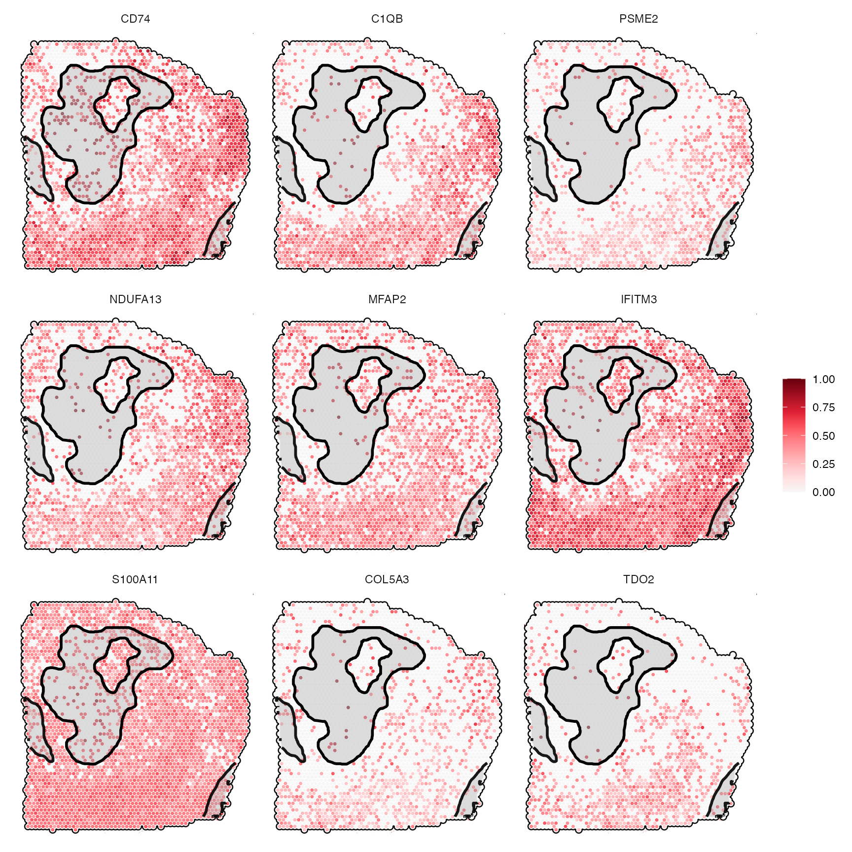

4. Pitfalls

There are some pitfalls regarding spatial annotation screening when it comes to setting up the screening parameters.

4.1 Incomplete annotation

Comprehensive annotation is important in order not to include areas in the screening that are actually of the same nature than the annotation (based on which the screening is conducted) itself. This would distort the pattern of the inferred gradient. For instance, compare the inferred gradient when disregarding the annotated necrotic area at the right bottom - labeled necrotic_edge. The distance parameter defines the maximum distance up to which observations are included in the screening. It defaults to the edge of the tissue (the maximal distance of all observations that were assigned to the tissue section it is located on).

all_necr_ids <- c("necrotic_area", "necrotic_edge", "necrotic_edge2")

# plot left, red outlines highlight the omitted annotations
plotSurface(object_t313, color_by = "VEGFA", display_image = F, pt_clrsp = "PuBu") + 
  ggpLayerSpatAnnOutline(object_t313, ids = "necrotic_area", fill = alpha("lightgrey", 0.25)) +
  # decrease resolution to 250um for visualization purpose 
  ggpLayerExprEstimatesSAS(object_t313, ids  = "necrotic_area", resolution = "250um") + 
  ggpLayerSpatAnnOutline(object_t313, ids = c("necrotic_edge", "necrotic_edge2"), line_size = 1.5, line_color = "red")

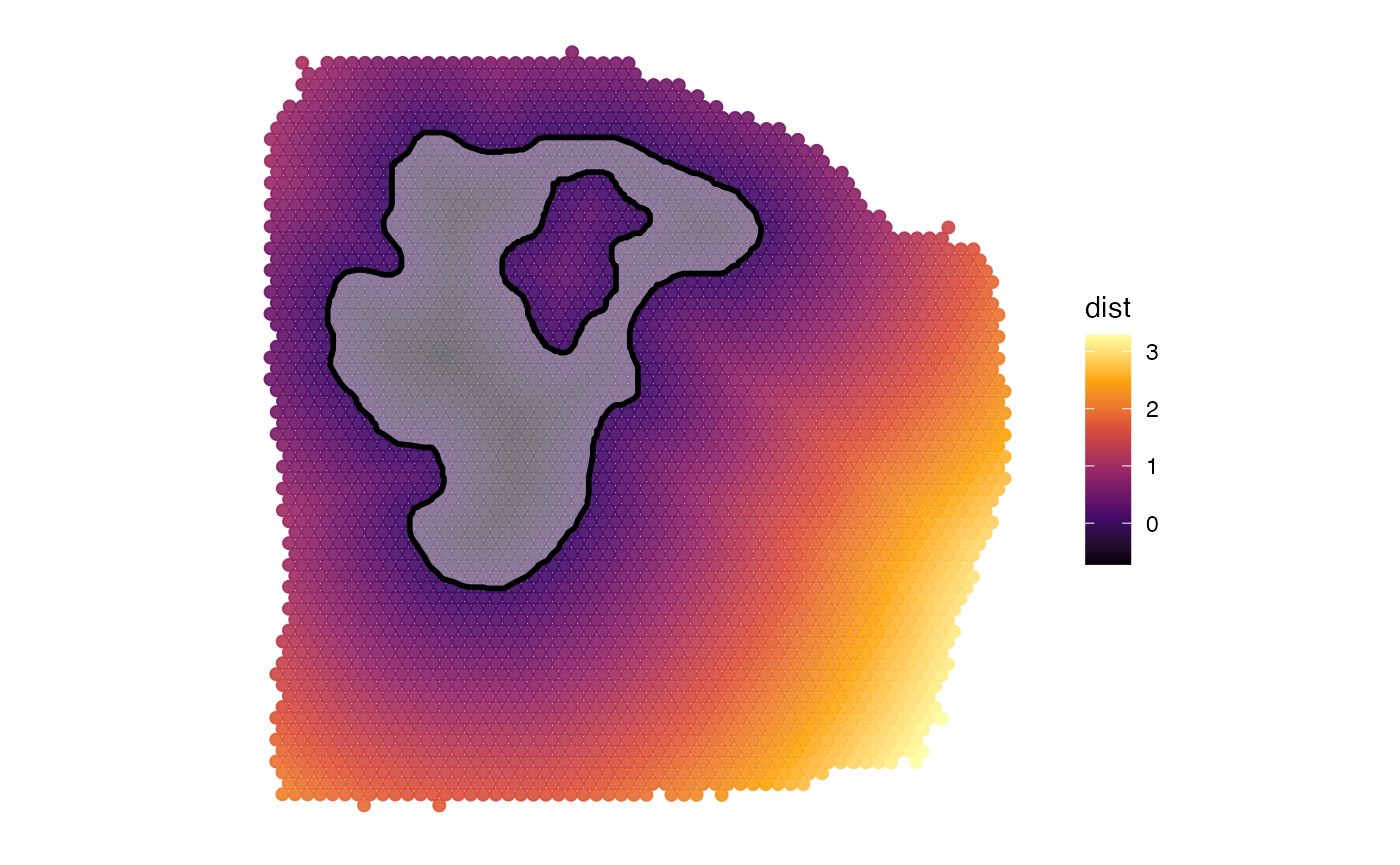
# plot right, distance = "dte": default
getCoordsDfSA(object_t313, ids = "necrotic_area", distance = "dte")  %>% 
  plotSurface(object = ., color_by = "dist", pt_clrsp = "inferno") + 
  ggpLayerSpatAnnOutline(object_t313, ids = "necrotic_area", fill = alpha("lightgrey", 0.25))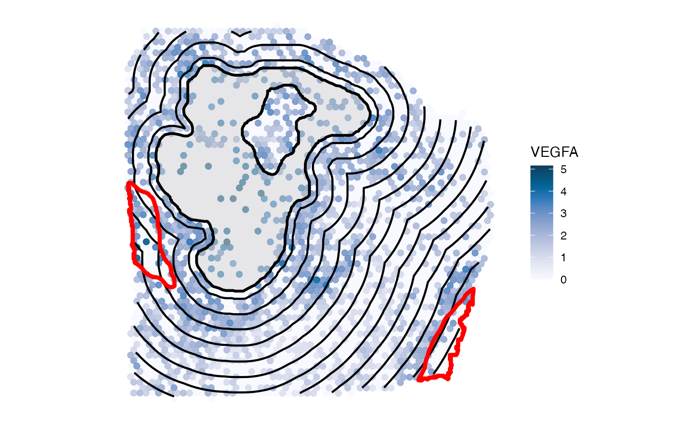

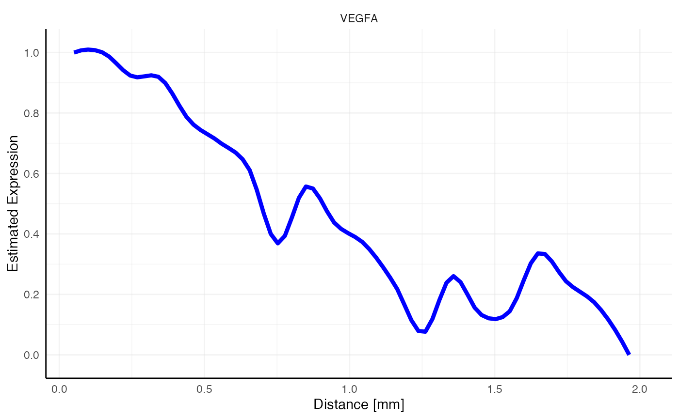
Suddenly, the gradient of VEGFA does not look as interesting as with all necrotic areas included. Note the peak at 2.7mm where the omitted necrotic edge is located. Therefore, make sure to include all areas in the screening set up that are big enough to have an impact on the screening results.

# plot left, only necrotic area, distance = "dte" screens the whole sample and includes other necrotic areas
plotSasLineplot(object_t313, variables = "VEGFA", ids = "necrotic_area", line_color = "blue") 

# plot right, comprehensive annotation as used in the example run above
plotSasLineplot(object_t313, variables = "VEGFA", ids = all_necr_ids, line_color = "blue")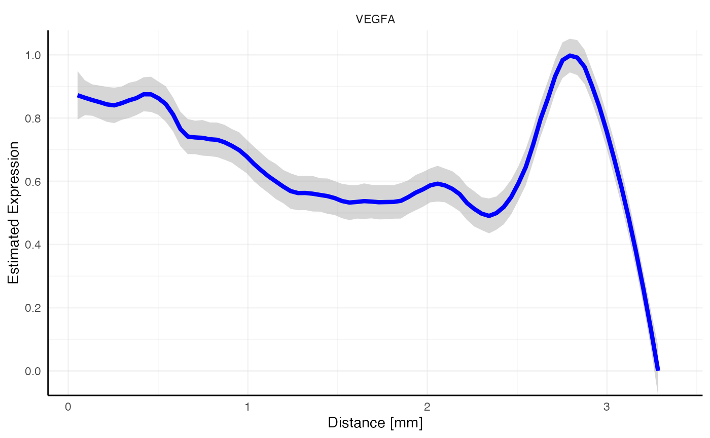

4.2 The tissue edge

Make sure that appropriate results of identifyTissueOutline() exist in the SPATA2 object. Consider the following sample of two mouse brain tissue sections with two stab wound injuries located in the cortex. While the clustering indicates a significant impact of these stab wounds on their local surrounding, this impact can logically only affect the tissue section they are located on. Inferring gene expression gradients up to a distance that transgresses the gab between both tissue sections can happen if the distance parameter is set carelessely and/or the tissue outline has not been identified properly!

# load injured mouse brain data 
object_mouse <- loadExampleObject("LMU_MCI", process = TRUE, meta = TRUE)

# "carelessly" set distance to "3mm"
dst <- "3mm"

# with tissue edge in mind (incl_edge = TRUE), only for inj1
expr_est_with_edge_in_mind <- 
  ggpLayerExprEstimatesSAS(object_mouse, ids = "inj1", incl_edge = T, distance = dst)

# without tissue edge in mind (incl_edge = FALSE), only for inj1
expr_est_without_edge_in_mind<- 
  ggpLayerExprEstimatesSAS(object_mouse, ids = "inj1", incl_edge = F, distance = dst)

# left plot
plotSurface(object_mouse, color_by = "clusters") + 
  ggpLayerSpatAnnOutline(object_mouse, ids = c("inj1", "inj2")) + 
  expr_est_with_edge_in_mind
  
# right plot
plotSurface(object_mouse, color_by = "clusters") + 
  ggpLayerSpatAnnOutline(object_mouse, ids = c("inj1", "inj2")) + 
  expr_est_without_edge_in_mind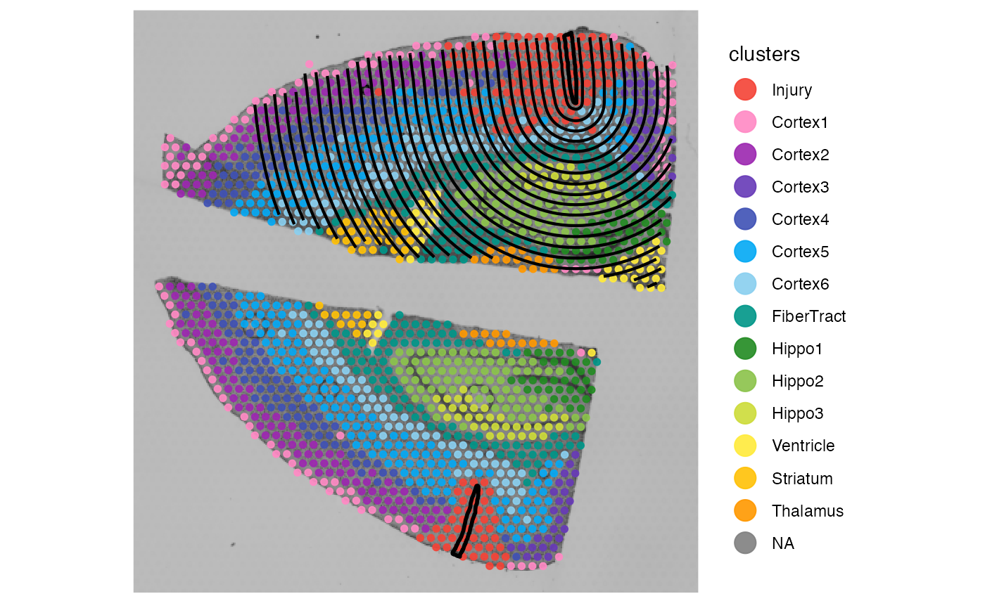

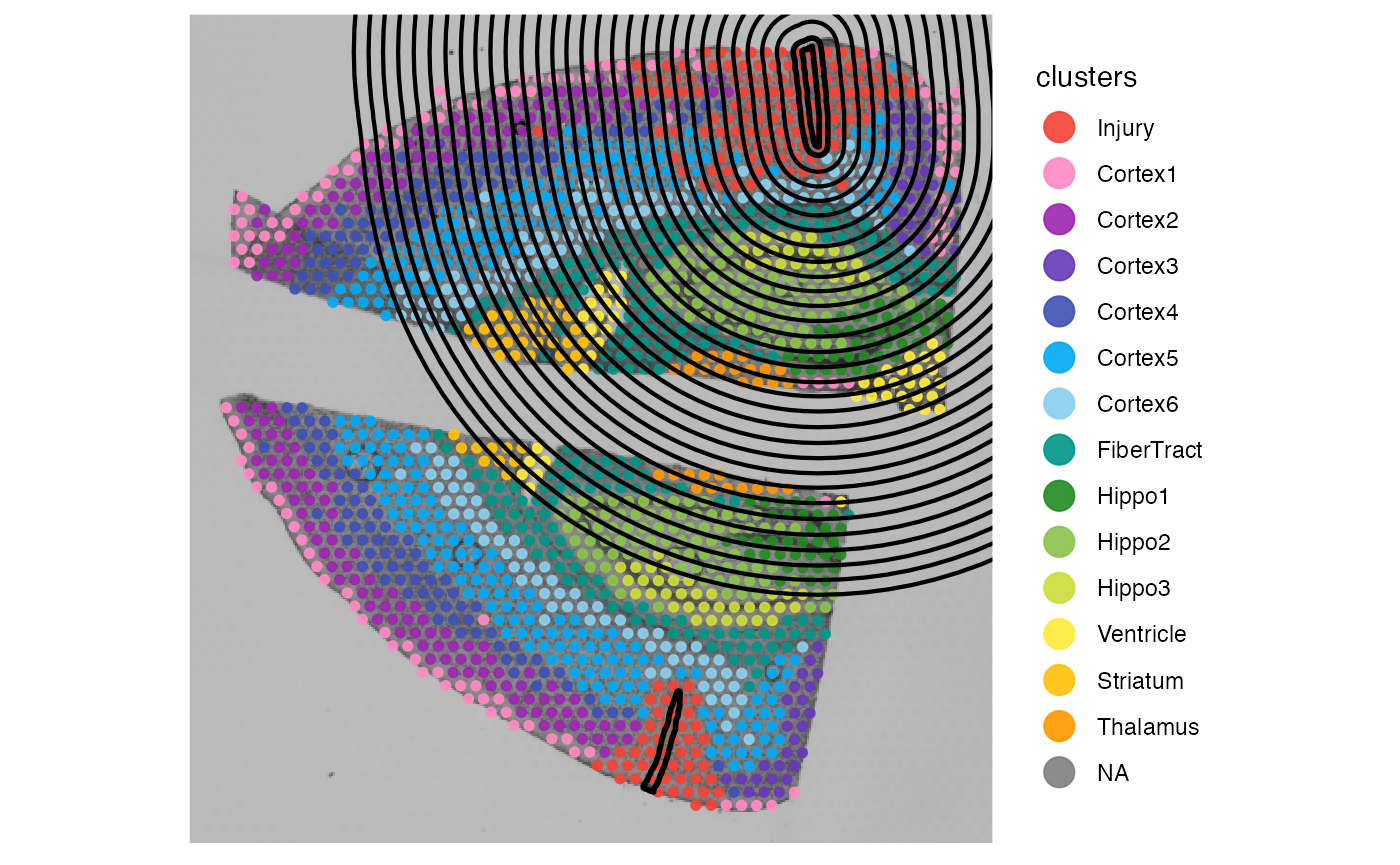
It goes without saying that the right plot displayes a screening set up that does not make sense. Gene expression would be estimated in regions that feature no tissue at all or in regions of a completely distinct tissue section with no biological connection to the spatial annotation of interest. Spatial annotation screening always makes sure that the screening does not transgresses the border of the tissue (in that sense, incl_edge is always TRUE). But to do that appropriately it requires proper results in the variable tissue_section as computed by identifyTissueOutline()!

# left plot
# color by the meta feature that just contains the sample name
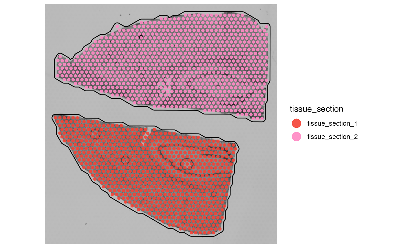
plotSurface(object_mouse, color_by = "sample")

# mess up the tissue_section variable manually 
object_mouse <- useVarForTissueOutline(object_mouse, var_name = "sample")

# right plot, distance = "3mm" transgresses the edge of the upper section
# because the two sections are not identified as separate sections
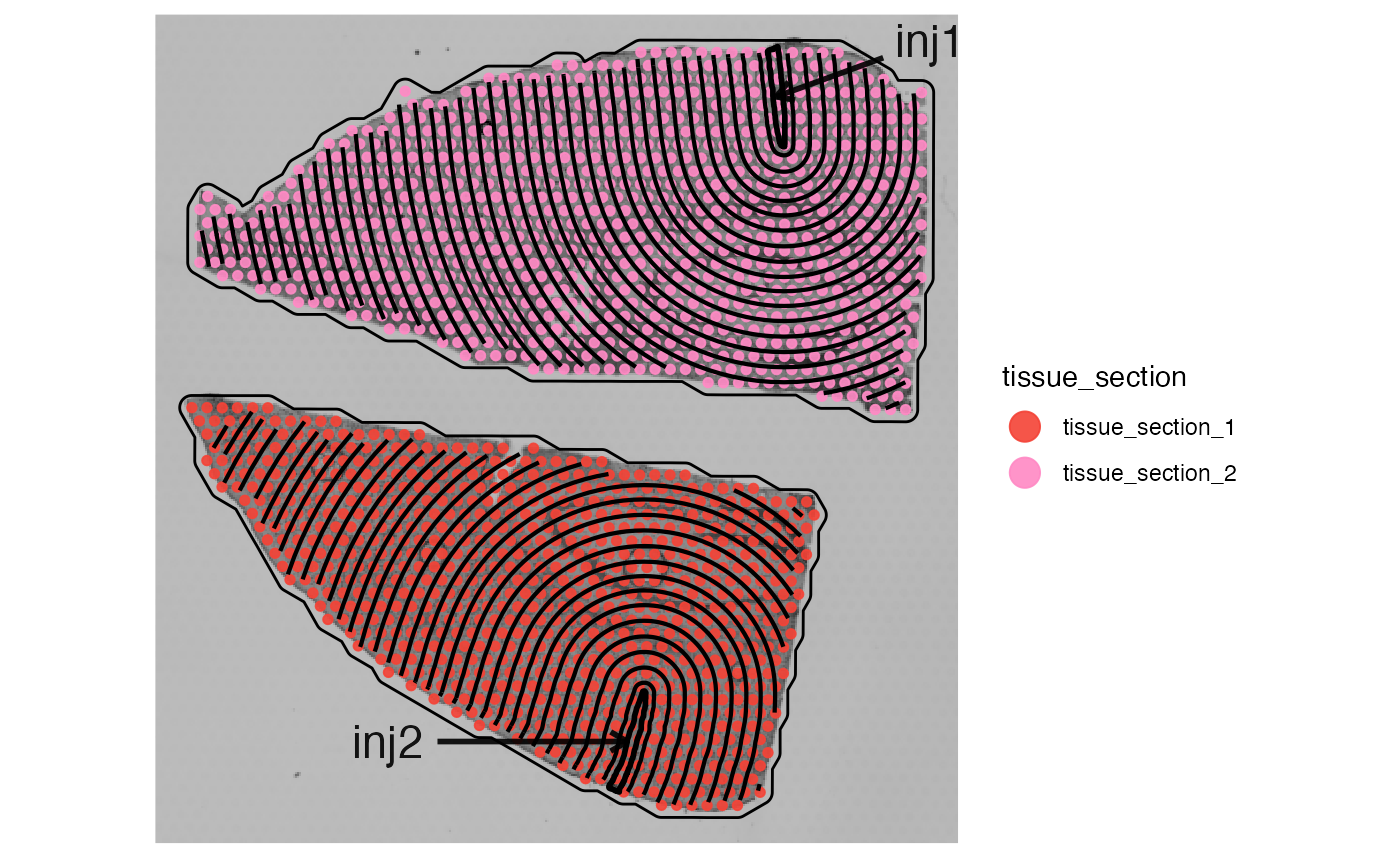
plotSurface(object_mouse, color_by = "tissue_section") + 
  ggpLayerExprEstimatesSAS(object_mouse, ids = "inj1", incl_edge = T, distance = dst)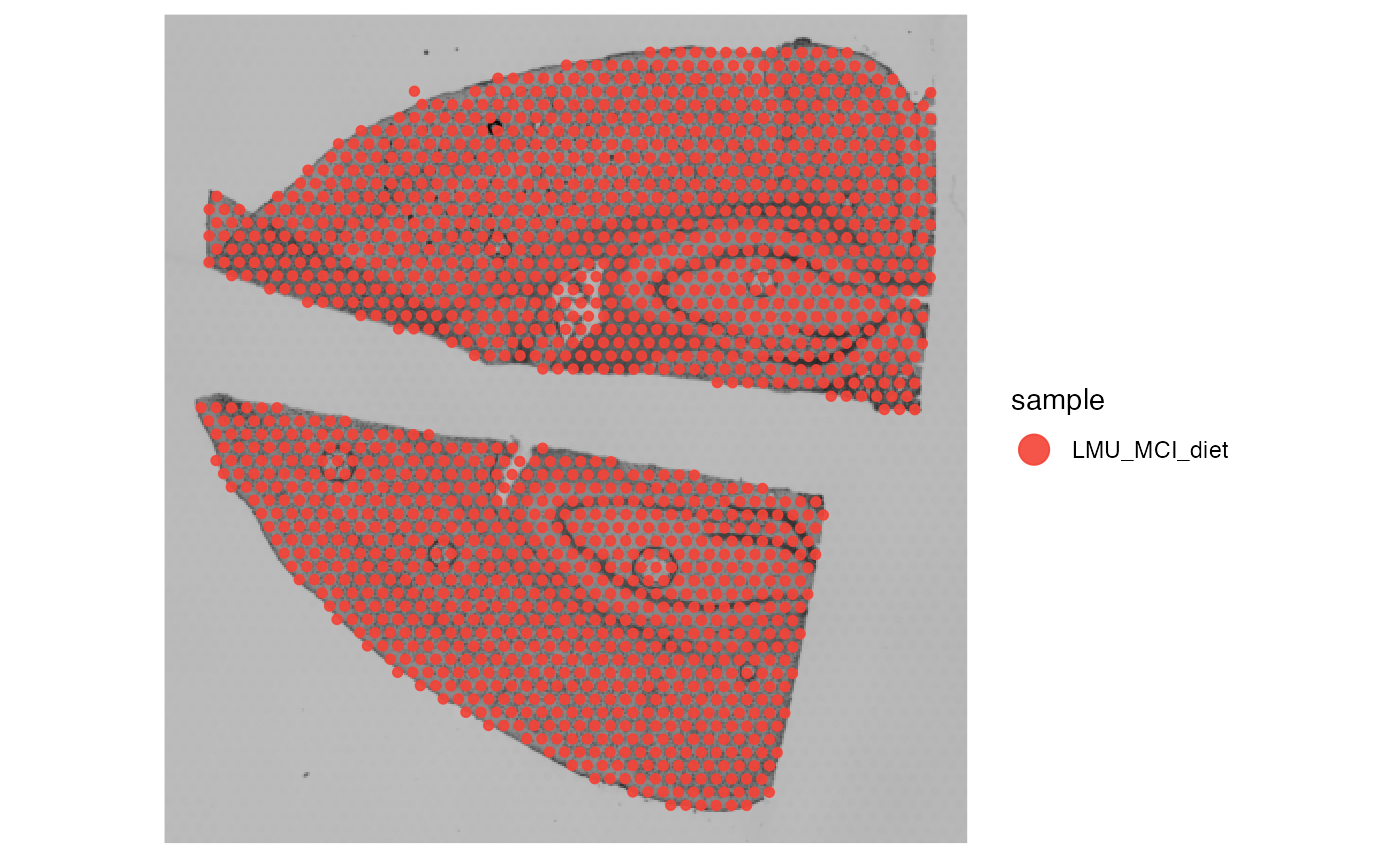

The right plot above shows that even if incl_edge is TRUE, the screening set up is nonsense because the information provided regarding the tissue outline and thus the tissue edge are messed up. Make sure that SPATA2 localizes the spatial annotations on the correct tissue sections and - in general - that tissue sections are correctly identified.

# overwrite tissue_section again
object_mouse <- identifyTissueOutline(object_mouse)

## 14:24:10 Identifying tissue outline with `method = obs`.

# check on which tissue sections the annotations are located on
whichTissueSection(object_mouse, id = "inj1")

## [1] "tissue_section_2"

whichTissueSection(object_mouse, id = "inj2")

## [1] "tissue_section_1"

# left plot
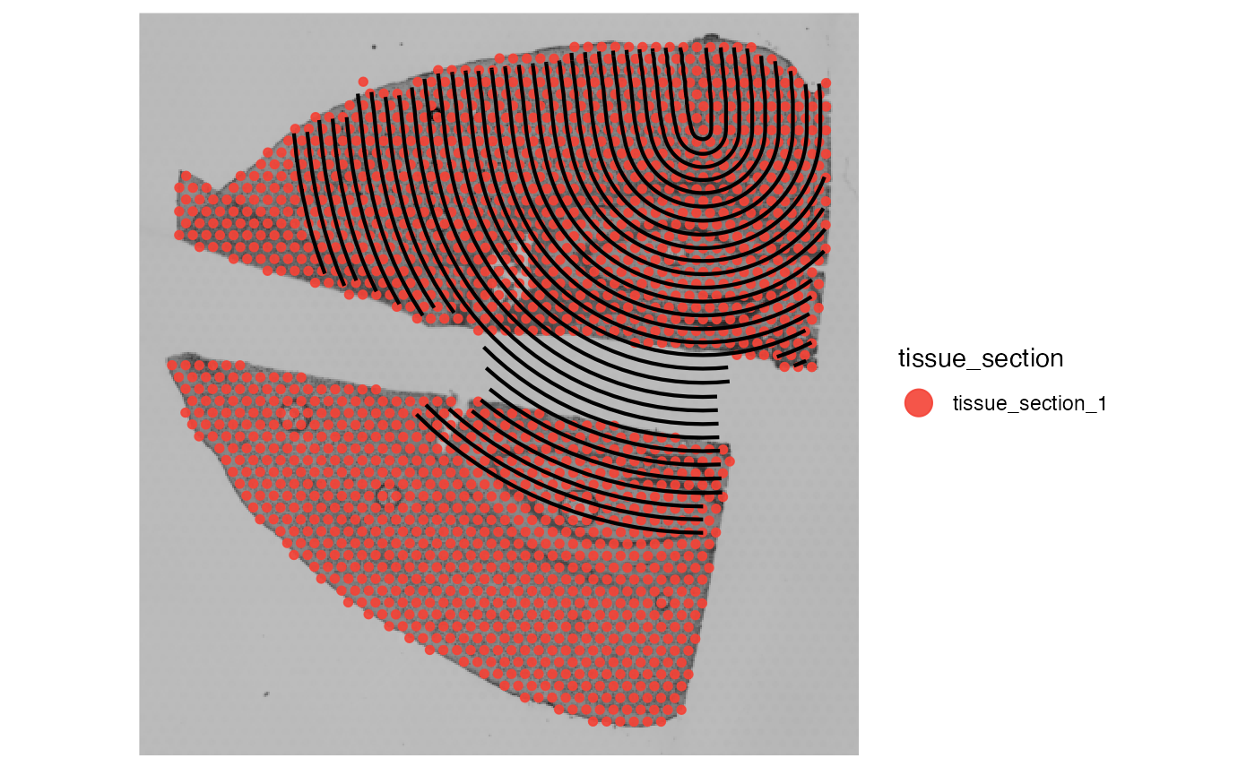
plotSurface(object_mouse, color_by = "tissue_section") + 
  ggpLayerTissueOutline(object_mouse)

# set the distance way too high
# -> no problem, since it is cut of at the tissue edge (which is now properly defined)
dst_high <- "10mm"

ids <- c("inj1", "inj2")

# right plot
# plot both annotations on the surface
# a warning informs you that the distance was adjusted based on the tissue edge
plotSurface(object_mouse, color_by = "tissue_section") + 
  ggpLayerTissueOutline(object_mouse, line_size = ) + 
  ggpLayerSpatAnnOutline(object_mouse, ids = ids) + 
  ggpLayerExprEstimatesSAS(object_mouse, ids = ids, incl_edge = T, distance = dst_high) +
  ggpLayerSpatAnnPointer(
    object = object_mouse, 
    ids = c("inj1", "inj2"),
    ptr_lengths = c("0.75mm", "1.25mm"),
    ptr_angles = c(70, 270),
    ptr_arrow = ggplot2::arrow(length = unit(0.1, "inches")), 
    text_dist = 25, 
    text_size = 6
    )

## Warning in get_coords_df_sa(object = object, id = id, distance = dist,
## resolution = resolution, : Parameter `distance` equals ~758.74px and exceeds
## the distance from spatial annotation 'inj1' to the edge of tissue section
## 'tissue_section_2' where it is located on: 298.74px. The parameter was adjusted
## accordingly.

## Warning in get_coords_df_sa(object = object, id = id, distance = dist,
## resolution = resolution, : Parameter `distance` equals ~758.74px and exceeds
## the distance from spatial annotation 'inj2' to the edge of tissue section
## 'tissue_section_1' where it is located on: 268.89px. The parameter was adjusted
## accordingly.