Initiation & Preprocessing Xenium
initiation-and-preprocessing-xenium.Rmd1. Introduction
This tutorial demonstrates how to load and preprocess Xenium data in
SPATA2 using the initiateSpataObjectXenium() function.
2. Load data
Here, we are using an exemplary mouse brain dataset from the 10X
Genomics website, downloaded 07/2024. The dataset for this tutorial
can be downloaded here. Save the folder on disk and
adjust the input for directory_merfish if necessary.
library(SPATA2)
library(SPATAData)
library(tidyverse)

# initiate the object from a folder directory
object <-
  initiateSpataObjectXenium(
     directory_merfish = "data/tutorial_initiate_xenium", # adjust to your liking
     sample_name = "hlcx" # h.uman l.ung c.ancer x.enium
   )
.
# output object
object
## An object of class SPATA2
## Sample: HumanLungCancerXenium
## Size: 162254 x 541 (cells x molecules)
## Memory: 183.05 Mb
## Platform: Xenium
## Molecular assays (1):
## 1. Assay
## Molecular modality: gene
## Distinct molecules: 541
## Matrices (1):
## -counts (active)
## Meta variables (2): sample, tissue_sectionWe obtained a SPATA2 object with 162,254 cells and 541
genes. The count matrix looks as follows:
# extract count matrix
count_mtr <- getCountMatrix(object)

# show results
count_mtr[10:15,1:5]
## 6 x 5 sparse Matrix of class "dgTMatrix"
## aaaadpbp-1 aaaaficg-1 aaabbaka-1 aaabbjoo-1 aaablchg-1
## ADH1C . . . . .
## ADH4 . . . . .
## ADIPOQ . . . . .
## AGER . . . . .
## AGR3 . . 1 . .
## AHSP . . . . .3. Spatial processing
First, we plot the cells colored by tissue section as identified by
identifyTissueOutline(). This function is called with
default parameters within initiateSpataObjectXenium(). If
the results of your objects are not satisfying adjust the parameters and
and run the function again. Every function call simply overwrites the
results. In this case, the default parameters worked out well and the
tissue outline as well as the section identification looks
appropriate.
# sets the default for this object
plotSurface(object, color_by = "tissue_section", pt_clrp = "milo") 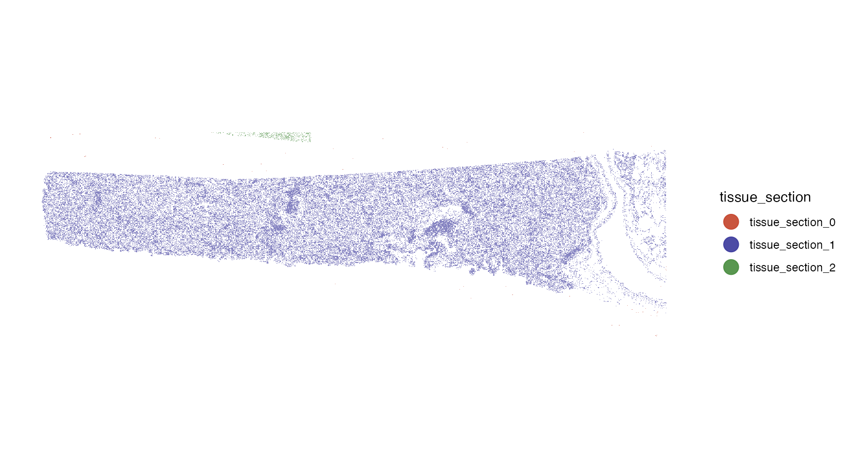
Seems as if there is a small fraction of cells that is not connected
to the main tissue section. Furthermore, there are cells that have not
been assigned to any tissue section (tissue_section_0). We can
identify and remove spatial outliers separated from the contiguous
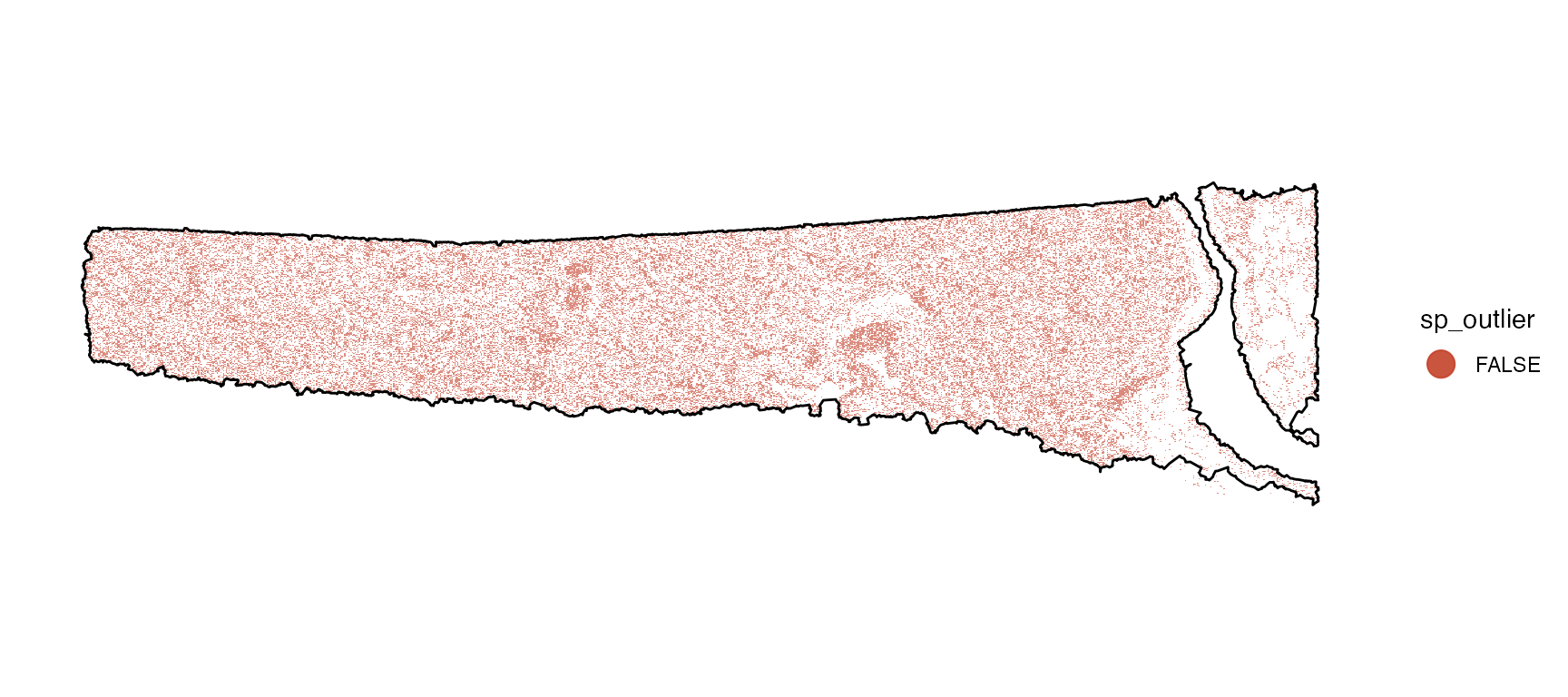
tissue section with identifySpatialOutliers(). Again, this
function runs on default parameters that can be adjusted. Refer to the
documentation for more information. In this case single outliers or
collection of cells of less than 5% of the overall number of cells (in
this case, 8112 cells) are considered spatial outliers. Running the
function creates a new column sp_outlier which is added to the
cell metadata.
# for some data.frame manipulation
library(dplyr)

# identify outliers based on the results of identifyTissueOutline()
object <- identifySpatialOutliers(object)
## 02:03:43 Identifying spatial outliers.## 02:03:43 Spatial outliers: 1149
# show the column
getCoordsDf(object, variables = "sp_outlier") %>%
  dplyr::filter(sp_outlier == TRUE) %>%
  select(barcodes, sample, sp_outlier, everything())
## # A tibble: 1,149 × 8
## barcodes sample sp_outlier x y x_orig y_orig cell_area
## <chr> <chr> <lgl> <dbl> <dbl> <dbl> <dbl> [um^2]
## 1 aaaadpbp-1 HumanLungCancerXen… TRUE 206. 1496. 206. 1496. 68.5
## 2 abfgiade-1 HumanLungCancerXen… TRUE 838. 3190. 838. 3190. 42.9
## 3 abfgkhjc-1 HumanLungCancerXen… TRUE 862. 3195. 862. 3195. 127.
## 4 abfgplcb-1 HumanLungCancerXen… TRUE 855. 3184. 855. 3184. 81.5
## 5 abfhjncf-1 HumanLungCancerXen… TRUE 848. 3183. 848. 3183. 34.0
## 6 aeejbbkm-1 HumanLungCancerXen… TRUE 269. 3516. 269. 3516. 33.3
## 7 aeejcmej-1 HumanLungCancerXen… TRUE 268. 3508. 268. 3508. 72.0
## 8 aeekonea-1 HumanLungCancerXen… TRUE 644. 3565. 644. 3565. 63.9
## 9 aghomlfd-1 HumanLungCancerXen… TRUE 2829. 3391. 2829. 3391. 67.0
## 10 ajcieihi-1 HumanLungCancerXen… TRUE 2559. 3131. 2559. 3131. 79.0
## # ℹ 1,139 more rowsThe results can be plotted with plotSurface().
# before
outline_with_outliers <- ggpLayerTissueOutline(object)

plot_with_outliers <-
  plotSurface(object, color_by = "sp_outlier", pt_clrp = "milo")

# remove the outliers
# note that with spatial_proc = TRUE (default), a new tissue outline is computed
object <- removeSpatialOutliers(object, spatial_proc = TRUE)

# afterwards
plot_without_outliers <-
  plotSurface(object, color_by = "sp_outlier", pt_clrp = "milo")

# plot top
plot_with_outliers +
  outline_with_outliers # old outline

# plot bottom
plot_without_outliers +
  ggpLayerTissueOutline(object) # new outline
4. Data processing
These steps are about additional noise removal as well as about processing raw counts.
4.1. Data cleaning
First you might want to remove certain genes from the raw count
matrix. There are wrappers for certain steps like
removeGenesStress() and
removeGenesZeroCounts(). Individual genes can always be
removed with removeGenes().
# before
nGenes(object)
## [1] 541

# removes stress genes
object <- removeGenesStress(object)

# removes genes that were not detected in any of the observations
object <- removeGenesZeroCounts(object)

# afterwards
nGenes(object)
## [1] 528
In some cases there are observations - in case of Visium barcoded
spots - left with no counts at all. If this is the case
removeObsZeroCounts() removes them. If there are none
nothing happens.
# before
nObs(object)
## [1] 161105

# check for and remove observations with zero counts
object <- removeObsZeroCounts(object)

# afterwards
nObs(object)
## [1] 160910
4.2 Matrix processing
The SPATA2 object is initiated with a raw count matrix.
For almost all downstream analysis steps it is recommended to use
processed matrices. The first step is usually log-normalization. To
create a normalized matrix use normalizeCounts(). It uses
Seurat::NormalizeData() in the background. The input
options for method correspond to the options in this
function from the Seurat package. By default, the normalized matrix is
named after input for method, activated and thus used by
default in downstream analysis and visualization. The function
normalizeCounts() can be called multiple times with
different inputs for method which populates the list of
processed matrices in the respective assay. Furthermore, processed
matrices can be added with addProcessedMatrix() if you want
to create them with SPATA2-extern functions. The default matrix that is
used can be set with activateMatrix(). By default,
normalizeCounts() activates the processed matrix it has
created. Here, we normalize using SCT as described in the Seurat
tutorial. This processes the raw count matrix. Results are stored in
the respective assays.
# no processed matrices, only raw counts
getProcessedMatrixNames(object)
## character(0)

getMatrixNames(object)
## [1] "counts"

activeMatrix(object)
## [1] "counts"

# normalize raw count data
# circumvent error with SCT???
object <- normalizeCounts(object, method = "LogNormalize")

# now the object contains normalized data
getProcessedMatrixNames(object)
## [1] "LogNormalize"

activeMatrix(object)
## [1] "LogNormalize"
By default, the normalized matrix is activated and thus used in
downstream analysis. See ?activateMatrix for more
information. Furthermore, we compute metadata for the cells:
n_counts_{modality} with molecular modality gene
represents the number of individual transcript counts per cell, whereas
n_distinct_{modality} represents the number of distinct genes
identified by cell.
# some more meta features
object <- computeMetaFeatures(object)

getMetaDf(object)
## # A tibble: 160,910 × 7
##    barcodes   sample     sp_outlier tissue_section n_counts_gene n_distinct_gene
##    <chr>      <chr>      <lgl>      <fct>                  <dbl>           <int>
##  1 aaaaficg-1 HumanLung… FALSE      tissue_sectio…            19              15
##  2 aaabbaka-1 HumanLung… FALSE      tissue_sectio…            53              38
##  3 aaabbjoo-1 HumanLung… FALSE      tissue_sectio…            29              18
##  4 aaablchg-1 HumanLung… FALSE      tissue_sectio…            43              34
##  5 aaacaicl-1 HumanLung… FALSE      tissue_sectio…           135              62
##  6 aaacfcef-1 HumanLung… FALSE      tissue_sectio…            61              32
##  7 aaacgpjg-1 HumanLung… FALSE      tissue_sectio…            12               9
##  8 aaacjhpm-1 HumanLung… FALSE      tissue_sectio…            61              34
##  9 aaacjlia-1 HumanLung… FALSE      tissue_sectio…            77              42
## 10 aaadbiaa-1 HumanLung… FALSE      tissue_sectio…            64              31
## # ℹ 160,900 more rows
## # ℹ 1 more variable: avg_cpm_gene <dbl>

# show overview (compare to overview above)
show(object)
## An object of class SPATA2
## Sample: HumanLungCancerXenium
## Size: 160910 x 528 (cells x molecules)
## Memory: 257.51 Mb
## Platform: Xenium
## Molecular assays (1):
## 1. Assay
##  Molecular modality: gene
##  Distinct molecules: 528
##  Matrices (2):
##  -counts
##  -LogNormalize (active)
## Meta variables (6): sample, sp_outlier, tissue_section, n_counts_gene, n_distinct_gene, avg_cpm_gene

# left plot
plotViolinplot(object, variables = c("n_counts_gene", "n_distinct_gene"))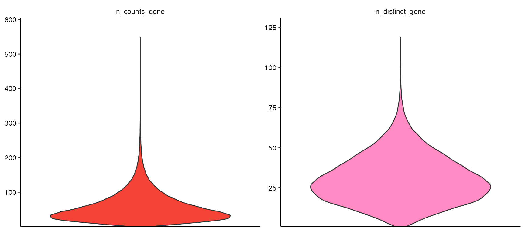
# upper plot
plotSurface(
  object = object,
  color_by = "n_counts_gene",
  limits = c(0, 200),
  oob = scales::squish,
  pt_clrsp = "Reds 3"
  ) +
  ggpLayerTissueOutline(object)

# lower plot
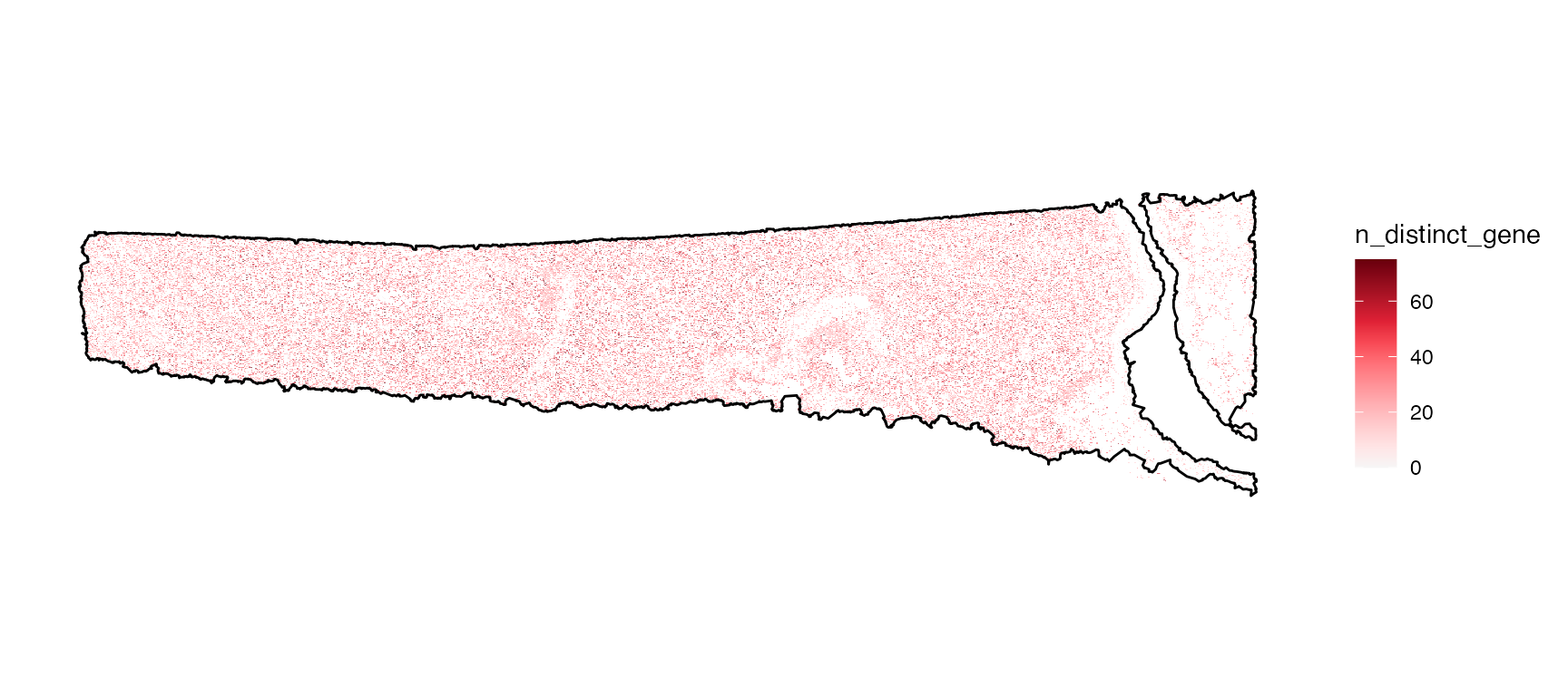
plotSurface(
  object = object,
  color_by = "n_distinct_gene",
  limits = c(0, 75),
  oob = scales::squish,
  pt_clrsp = "Reds 3"
  ) +
  ggpLayerTissueOutline(object)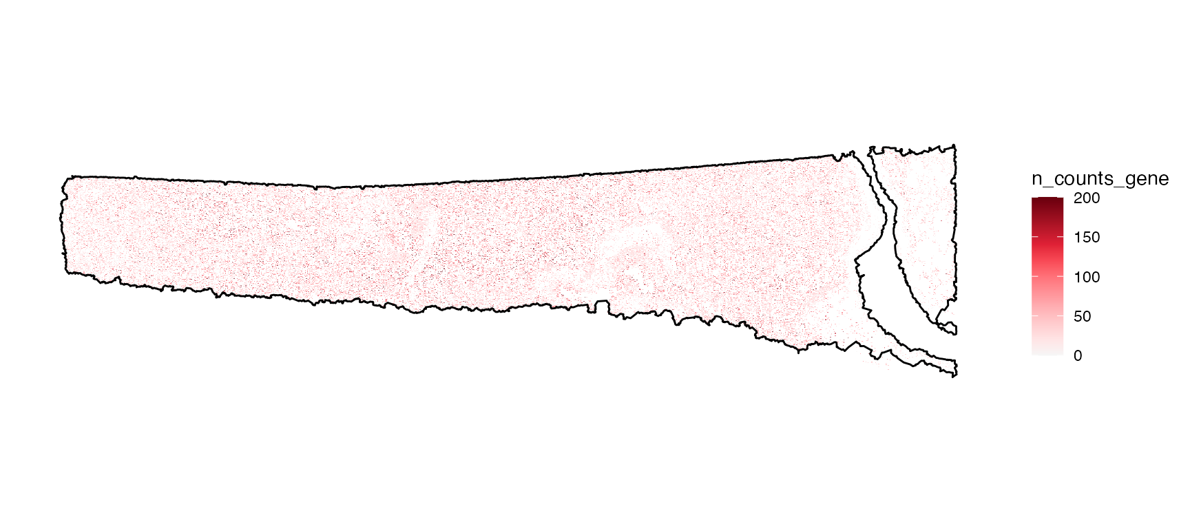
5. Spatially variable genes
Next, we identify spatially variable genes using SPARK-X.
# run the algorithm
object <- runSPARKX(object)
## ## ===== SPARK-X INPUT INFORMATION ====
## ## number of total samples: 160910
## ## number of total genes: 528
## ## Running with single core, may take some time
## ## Testing With Projection Kernel
## ## Testing With Gaussian Kernel 1
## ## Testing With Gaussian Kernel 2
## ## Testing With Gaussian Kernel 3
## ## Testing With Gaussian Kernel 4
## ## Testing With Gaussian Kernel 5
## ## Testing With Cosine Kernel 1
## ## Testing With Cosine Kernel 2
## ## Testing With Cosine Kernel 3
## ## Testing With Cosine Kernel 4
## ## Testing With Cosine Kernel 5
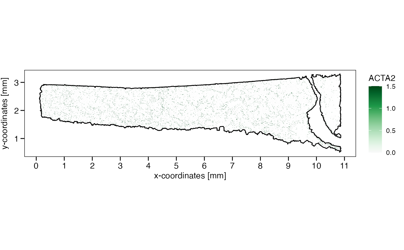
sparkx_genes <- getSparkxGenes(object, threshold_pval = 0.05)

str(sparkx_genes)
##  chr [1:362] "ACE2" "ACTA2" "BASP1" "BCL2L11" "CAPN8" "CD79A" "CFTR" "CNN1" ...

# add axes labeling in SI units with customized breaks
axes_layer <- ggpLayerAxesSI(object, breaks = list(x = str_c(0:11, "mm"), y = str_c(1:3, "mm")))

# left plot
plotSurface(object, color_by = sparkx_genes[1], pt_clrsp = "Purple-Blue") +
  axes_layer +
  ggpLayerTissueOutline(object) # use outline to plot against white

# right plot (set the color scale limits)
plotSurface(object, color_by = sparkx_genes[2], pt_clrsp = "Greens 3", limits = c(0, 1.5), oob = scales::squish) +
  axes_layer +
  ggpLayerTissueOutline(object)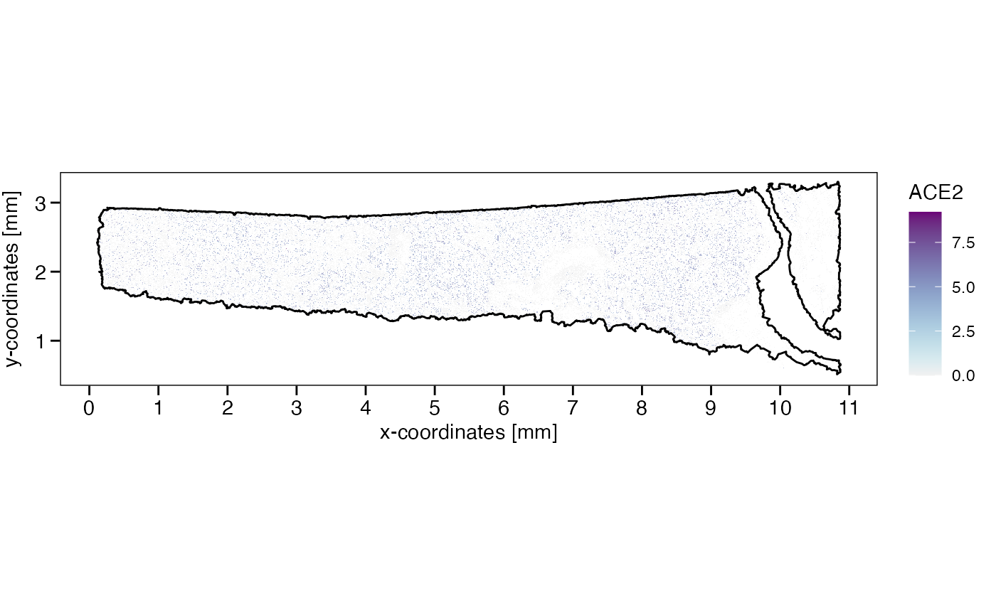
6. Subset observations
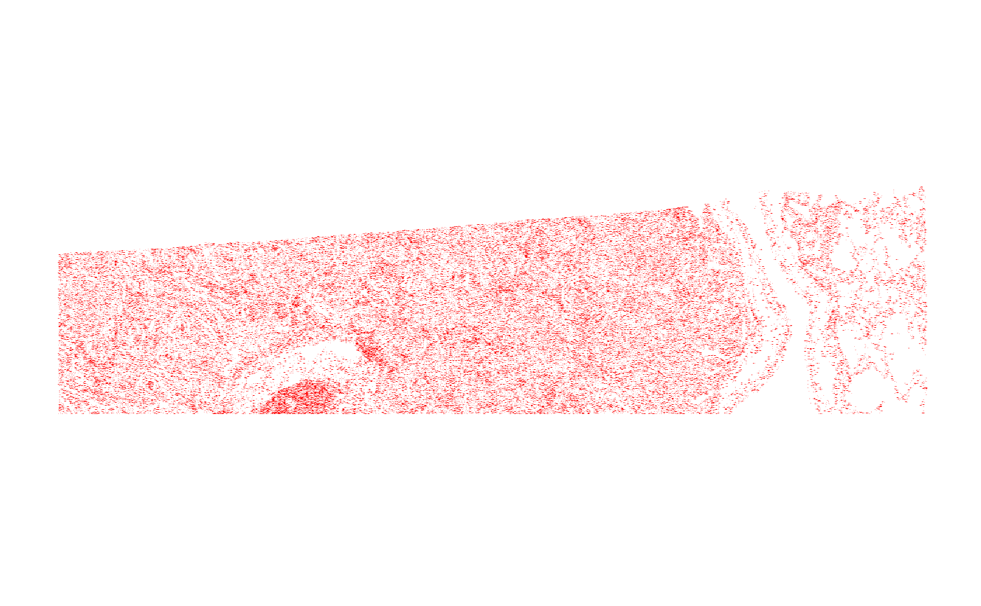
For examples, we provide a small example object. Here, we additionally subset the dataset to just extract the top right corner.
# get range of upper right corner
crop_range <-
  getCoordsRange(object) %>%
  purrr::map(.f = ~ c(mean(.x), max(.x)))

# show results
crop_range
## $x
## [1]  5493.139 10873.031
##
## $y
## [1] 1895.419 3302.554

p_before <-
  plotSurface(object, pt_clr = "red") +
  ggpLayerTissueOutline(object) +
  ggpLayerRect(object, xrange = crop_range$x, yrange = crop_range$y)

# crop with a rectangular
object_subset <- cropSpataObject(object, xrange = crop_range$x, yrange = crop_range$y)

p_subset <- plotSurface(object_subset, pt_clr = "red")

# left plot
p_before

# right plot
p_subset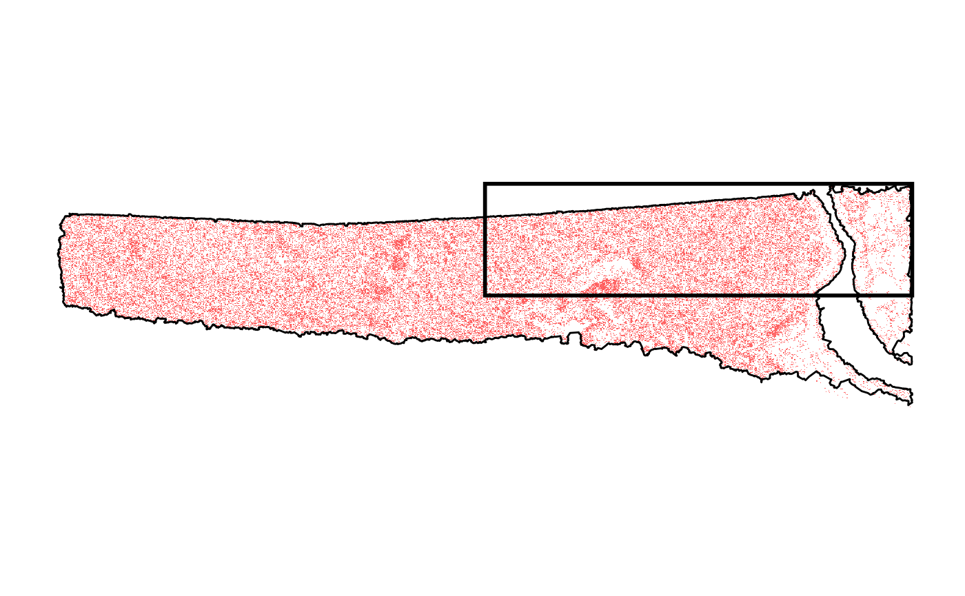
6. Conclusion and more data sets
That’s it. The object can be used for any downstream analyses such as dimensional reduction, clustering, spatial annotation screening or spatial trajectory screening. Refer to tab Tutorials for more links. Furthermore, you can skim our curated data base of spatial data sets for those of platform Xenium using SPATAData.
# load package
library(SPATAData)

# filter for samples from platform VisiumHD
sourceDataFrame(platform == "Xenium")
## # A tibble: 0 × 0