Prerequisites
Make sure to be familiar with the following tutorials before proceeding:
1. Introduction
Dimensional reduction is an important step in visualizing the heterogeneity of your data. In cypro it is conducted based on variable sets. It explains how you can conduct Principal Component Analysis, TSNE and UMAP reductions and visualize the results.
2. Computation
A set of intensity related variables will serve as an example.
# show variables of a previously defined variable set
getVariableSet(object, variable_set = "intensity")
output
##  [1] "Intensity_LowerQuartileIntensity_Actin"
##  [2] "Intensity_MADIntensity_Actin"
##  [3] "Intensity_MassDisplacement_Actin"
##  [4] "Intensity_MaxIntensityEdge_Actin"
##  [5] "Intensity_MaxIntensity_Actin"
##  [6] "Intensity_MeanIntensityEdge_Actin"
##  [7] "Intensity_MeanIntensity_Actin"
##  [8] "Intensity_MedianIntensity_Actin"
##  [9] "Intensity_MinIntensityEdge_Actin"
## [10] "Intensity_MinIntensity_Actin"
## [11] "Intensity_UpperQuartileIntensity_Actin"
There is a function for every algorithm respectively. runPca(), runTsne() and runUmap().
object <- runPca(object, variable_set = "intensity")

object <- runUmap(object, variable_set = "intensity")
Dimensional reduction is part of the overall analys module in cypro. Use printAnalysisSummary() to get an overview about the dimensional reduction you have calculated for the variable sets in your cypro object.
# tsne is missing as it hasn't been computed yet
printAnalysisSummary(object, slots = "dim_red")
output
##
## --------------------------------------------------
##
## Conducted analysis:
##
##
##
##
## |dim_red |intensity |area |
## |:-------|:---------|:----|
## |pca     |Yes       |No   |
## |tsne    |No        |No   |
## |umap    |Yes       |No   |
##
##
##
## --------------------------------------------------
3. Visualisation
Again, there is a function for every algorithm respectively. They come with a variety of options with which you can tweak the plots.
plotPca(object,
        variable_set = "intensity",
        color_by = "condition",
        pt_size = 1)

plotPca(object,
        variable_set = "intensity",
        color_by = "Intensity_MaxIntensity_Actin",
        pt_size = 1)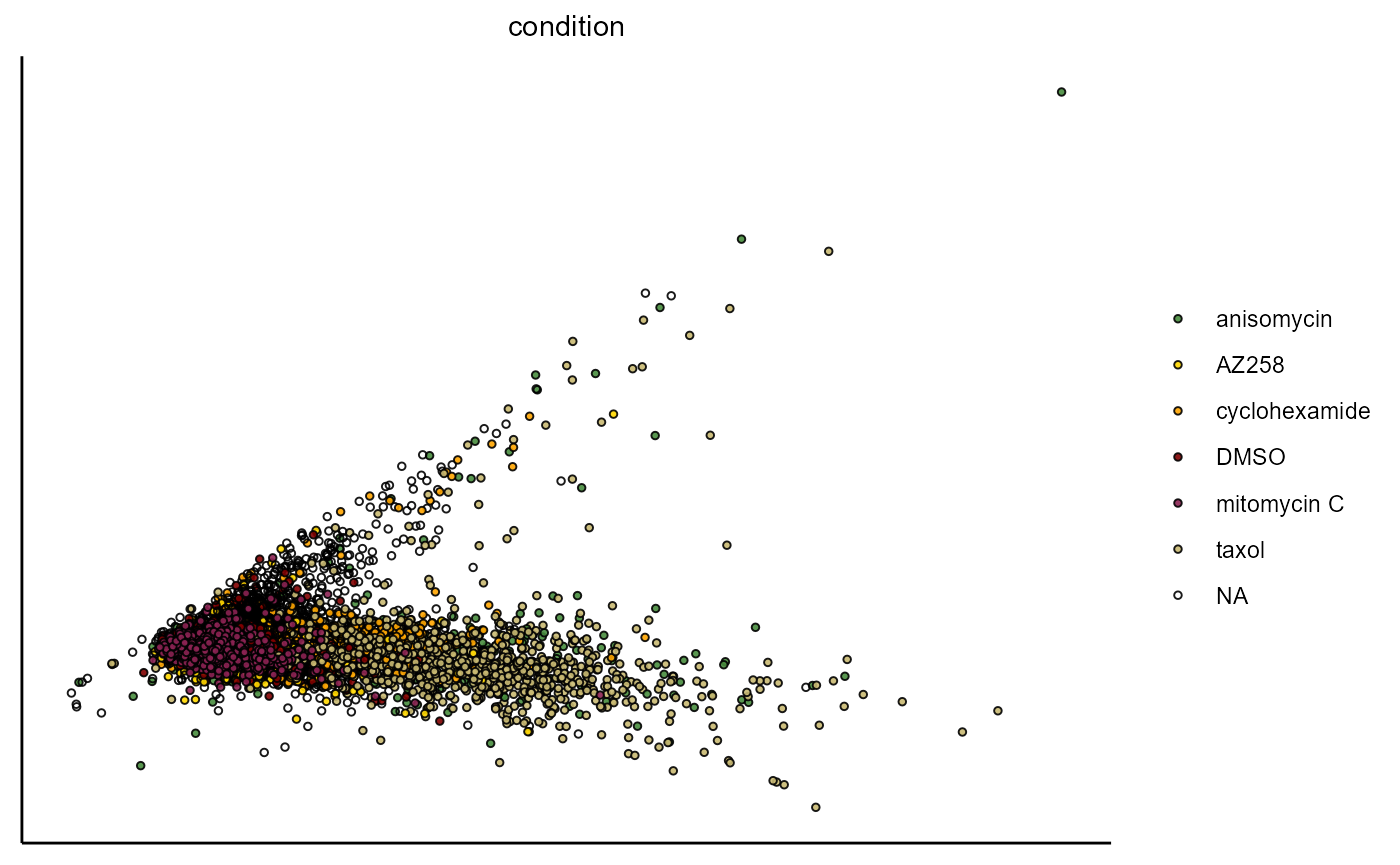
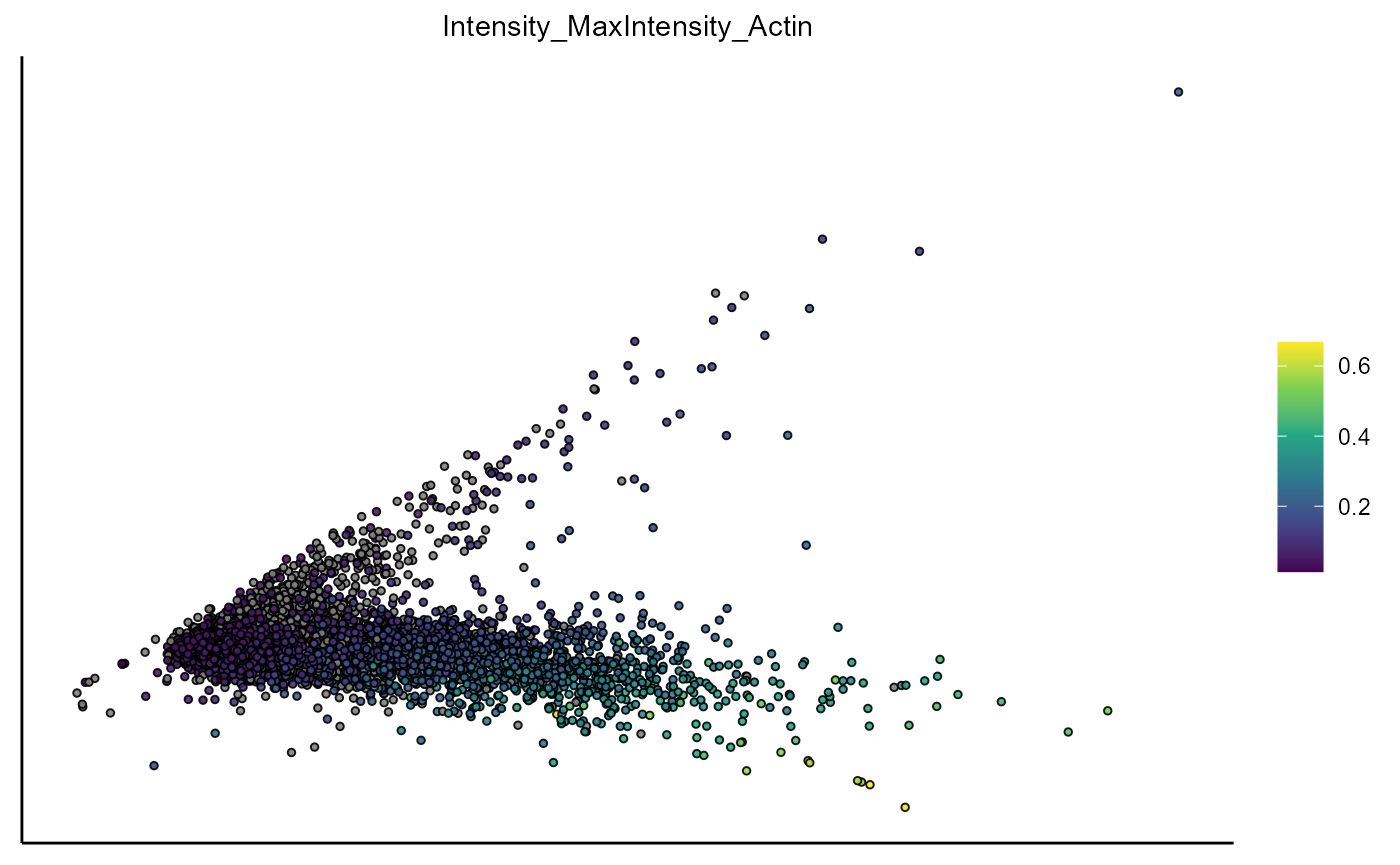
Figure 1.1 Visualization of PCA based on the variable set ‘intensity’
plotUmap(object,
         variable_set = "intensity",
         color_by = "condition",
         pt_size = 1)

plotUmap(object,
         variable_set = "intensity",
         color_by = "kmeans_Lloyd_k_4_(intensity)",
         pt_size = 1)
## Color palette 'milo' contains only 4 values. Need 5. Using default color clrp.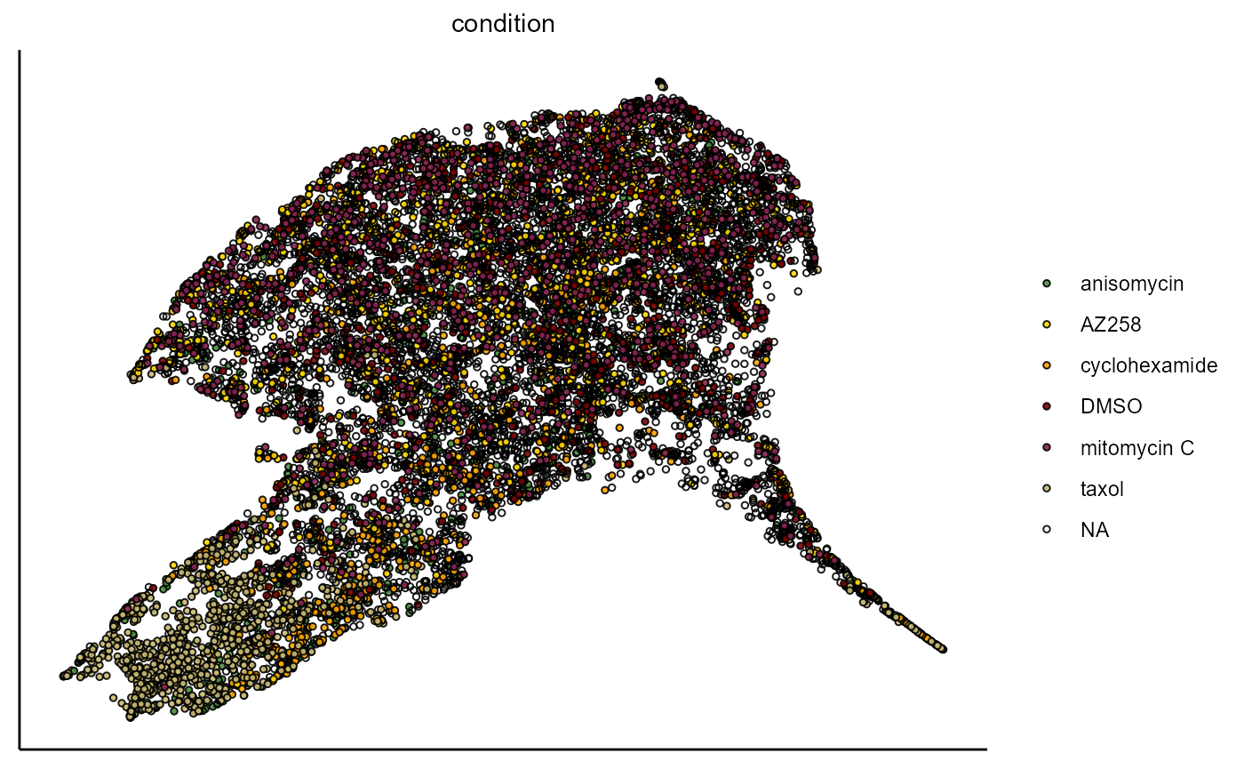
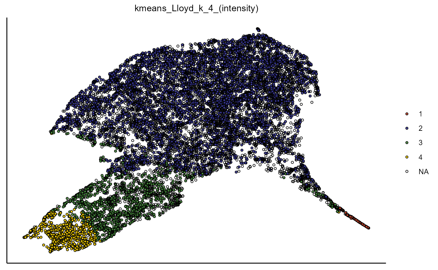
Figure 1.2 Visualization of UMAP embedding based on the variable set ‘intensity’
4. Extraction
Dimensional reduction is stored in the @analysis-slot under $dim_red. Every dimensional reduction for every variable set is stored in a specific S4-object as programmed in the package confuns called dim_red_conv. Use the respective function getPcaObject(), getTsneObject(), getUmapObject() to extract the S4-objects containing all data needed to proceed with the analysis on your own terms.