Clustering • cypro

Prerequisites

Make sure to be familiar with the following tutorials before proceeding:

Variable Sets

1. Introduction

There are a variety of clustering algorithms. Each of these algorithms comes with its own specific methods and options and metrics such as different distance measures (euclidean, manhattan) or agglomeration methods (complete, ward.D). As clustering is exploratory approach more than one way of clustering cells might be correct or at least provide a satisfying model. cypro currently implements hierarchical, kmeans and partitioning around medoids (PAM). It does that in a convenient fashion that allows you to iterate over a variety of clustering options for a variety of variable sets and to store all results in the cypro object - ready to be plotted or extracted when needed. This tutorial introduces you to the workflow of all three clustering methods.

# load packages
library(cypro)

# load object from broad institute compound profiling experiment week 4
# contains one time imaging data
object <- readRDS(file = "data/bids-week4.RDS")

2. Hierarchical clustering

Hierarchical clustering is one of the most common algorithms used in exploratory data analysis. It usually contains four steps:

1. Decide which data variables you want to base the clustering on.
1. Compute a distance matrix based on the data variables (several distance metrics exist).
1. Agglomerate the observations to a hierarchical tree based on the distance matrix (several agglomeration metrics exist).
1. Cut the hierarchical tree at a certain height or with a certain predefined value for k.

The cypro package implements these four steps with four functions.

2.1 Initiation

To initiate hierarchical clustering means to set up the respective S4 object in your cypro object by determining the variables on which you want to base the clustering. This is done with cypros variable set functionality.

# show variables of a previously defined variable set
getVariableSet(object, variable_set = "intensity")

output

##  [1] "Intensity_LowerQuartileIntensity_Actin"
##  [2] "Intensity_MADIntensity_Actin"          
##  [3] "Intensity_MassDisplacement_Actin"      
##  [4] "Intensity_MaxIntensityEdge_Actin"      
##  [5] "Intensity_MaxIntensity_Actin"          
##  [6] "Intensity_MeanIntensityEdge_Actin"     
##  [7] "Intensity_MeanIntensity_Actin"         
##  [8] "Intensity_MedianIntensity_Actin"       
##  [9] "Intensity_MinIntensityEdge_Actin"      
## [10] "Intensity_MinIntensity_Actin"          
## [11] "Intensity_UpperQuartileIntensity_Actin"

The function initiateHierarchicalClustering() prepares the clustering within the cypro object.

object <- initiateHierarchicalClustering(object, variable_set = "intensity")

2.2 Compute distance matrices

To obtain all valid methods with which distance matrices can be computed use validDistanceMethods().

validDistanceMethods()

## [1] "euclidean" "maximum"   "manhattan" "canberra"  "binary"    "minkowski"

While you can specify the distance methods one by one, a more convenient approach would be to tell cypro all distance metrics of interest and then let it do the computation for each one respectively in one function call.

distance_methods <- c("euclidean", "manhattan")

object <- computeDistanceMatrices(object, variable_set = "intensity", method_dist = distance_methods)

2.3 Agglomerate hierarchical cluster

There are a variety of methods to agglomerate distance measures to hierarchical tree. Again you can specify all approaches you would like to explore in one simple function call. Use validAgglomerationMethods() to obtain valid input options for argument method_aggl.

validAgglomerationMethods()

## [1] "ward.D"   "ward.D2"  "single"   "complete" "average"  "mcquitty" "median"  
## [8] "centroid"

Specifying two different input options makes agglomerateHierarchicalCluster() use every unique combination automatically.

aggl_methods <- c("complete", "ward.D")

object <- 
  agglomerateHierarchicalCluster(
    object = object,
    variable_set = "intensity",
    method_dist = distance_methods,
    method_aggl = aggl_methods
    )

The function plotDendrogram() allows to visualize cluster agglomeration with a variety of options. Check out its documentation with ?plotDendrogram.

plotDendrogram(object, variable_set = "intensity", method_dist = "euclidean", method_aggl = "ward.D", k = 4)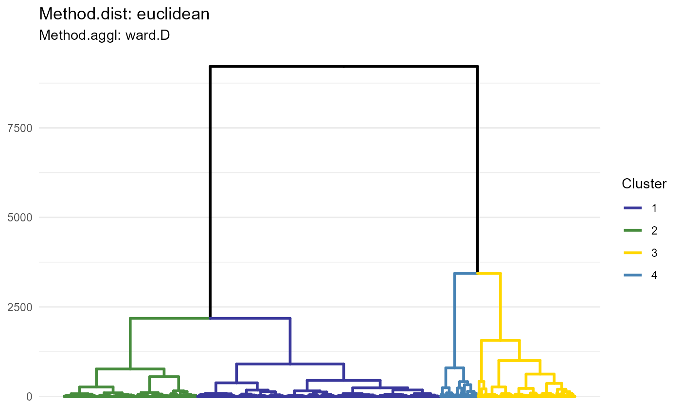

Figure 1.1 Dendrogram visualizing one of the distance-agglomeration options

2.4 Adding hierarchical cluster variables

To make interesting clustering results available for subsequent analysis steps they must be added in form of grouping variables to the cluster data. If no variables have been added the data.frame is empty.

# no clustering variables have been added yet
getClusterVariableNames(object)

## No cluster variables have been calculated yet.

## character(0)

Adding clustering variables can be done conveniently via addHierarchicalClusterVariables(). Specify distance methods, agglomeration methods and all ways according to which you want to cut the trees. All valid combinations are added to the cell cluster data and are made available for arguments like across or grouping_variable.

object <- 
  addHierarchicalClusterVariables(
    object = object,
    variable_set = "intensity",
    method_dist = "euclidean",
    method_aggl = c("complete", "ward.D"),
    k = c(3,4,5)
    )

getClusterVariableNames(object)

## [1] "hcl_euclidean_complete_k_3_(intensity)"
## [2] "hcl_euclidean_complete_k_4_(intensity)"
## [3] "hcl_euclidean_complete_k_5_(intensity)"
## [4] "hcl_euclidean_ward.D_k_3_(intensity)"  
## [5] "hcl_euclidean_ward.D_k_4_(intensity)"  
## [6] "hcl_euclidean_ward.D_k_5_(intensity)"

2.5 A note on handling distance matrices

Distance matrices can become very big in size. The convenient iteration that cypro allows comes with a drawback: The cypro object grows in size pretty quick, too.

pryr::object_size(object)

## 1.41 GB

hclust_conv <- getHclustConv(object, variable_set = "intensity")

euclidean_dist_mtr <- hclust_conv@dist_matrices$euclidean

pryr::object_size(euclidean_dist_mtr)

## 677 MB

Fortunately, the computation of distance matrices and the agglomeration of hierarchical cluster are separated processes. Once the hierarchical tree has been agglomerated based on a distance matrix, the latter is not needed any longer. You can therefore discard distance matrices, even before adding the cluster variables to the cell data.

object <- discardDistanceMatrix(object, variable_set = "intensity", method_dist = "euclidean")

hclust_conv <- getHclustConv(object, variable_set = "intensity")

# does not exist any longer ( == NULL)
hclust_conv@dist_matrices$euclidean

## NULL

# cypro object is way smaller 
pryr::object_size(object)

## 738 MB

We recommend to regularly check the size of the cypro object with pryr::object_size() and to discard unneeded distance matrices. In case you realize after discarding that you need it again you can always compute it again via computeDistanceMatrices() without initiating a new hierarchical clustering for the variable set of interest!

3. Kmeans clustering

Kmeans clustering can be conducted in a similar fashion.

3.1 Initiatiation

To initiate kmeans clustering based on a new variable set use initiateKmeansClustering().

object <- initiateKmeansClustering(object, variable_set = "intensity")

3.2 Cluster computation

validKmeansMethods() provides all valid kmeans methods.

validKmeansMethods()

## [1] "Hartigan-Wong" "Lloyd"         "Forgy"         "MacQueen"

The function computeKmeansCluster() iterates over all valid input combinations for arguments k and method_kmeans.

kmeans_methods <- c("Hartigan-Wong", "Lloyd")

object <- 
  computeKmeansCluster(
    object = object,
    variable_set = "intensity",
    k = 2:10, # compute clustering for values k = 2, k = 3, ... k = 10
    method_kmeans = kmeans_methods
    )

To assess clustering quality and optimal inputs for k use plotScreeplot(). Based on it’s output you can decide with which clustering results you want to proceed.

plotScreeplot(object, variable_set = "intensity", k = 2:10, method_kmeans = kmeans_methods)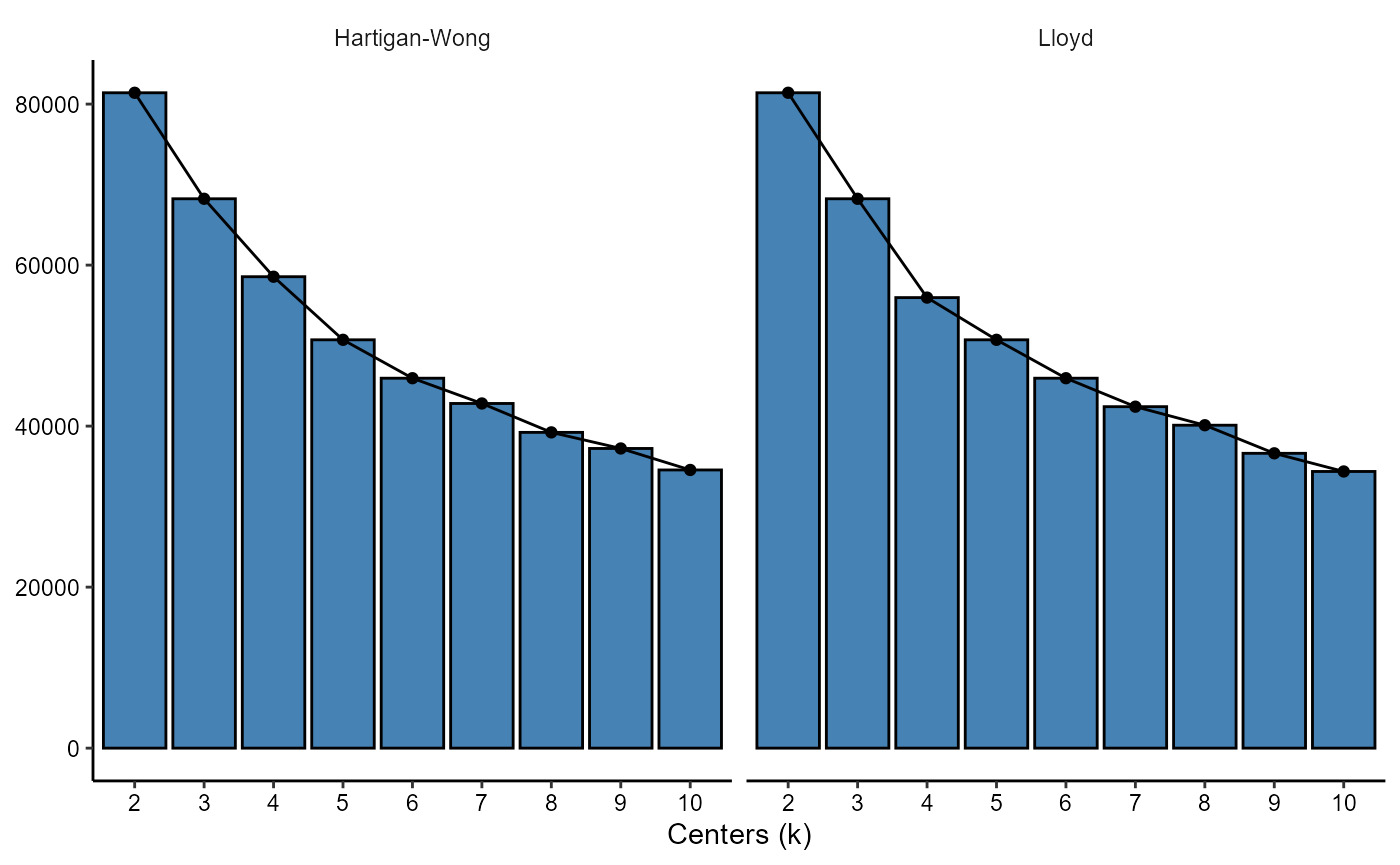

Figure 3.1 Screeplots can be used to determine optimal value for k

3.4 Adding kmeans cluster variables

To make clustering results available for subsequent functions use addKmeansClusteringVariables().

object <- addKmeansClusterVariables(object, variable_set = "intensity", k = 3:5, method_kmeans = "Lloyd")

getClusterVariableNames(object, starts_with("kmeans"))

## [1] "kmeans_Lloyd_k_3_(intensity)" "kmeans_Lloyd_k_4_(intensity)"
## [3] "kmeans_Lloyd_k_5_(intensity)"

4. Partitioning around medoids (PAM)

The PAM algorigthm works very similar to kmeans although it is a bit more robust and comes with an additional metric, silhouette width, to assess cluster quality. A major drawback of this algorithm: It is way slower than kmeans. A recommended approach is to conduct kmeans clustering first to narrow down the values for argument k that come into question. Apart from that the PAM clustering workflow is equal to the one of kmeans.

4.1 Initiate PAM clustering

Use the function initiatePamClustering() to set up the analysis pipeline with the set of data variables you want to base the clustering on.

object <- initiatePamClustering(object, variable_set = "intensity")

4.2 Run the algorithm

… with function computePamCluster().

object <- computePamCluster(object, variable_set = "intensity", k = 2:10)

Partitioning around medoids comes with some plotting options to assess cluster quality such as the average silhouette width…

plotAvgSilhouetteWidths(object, variable_set = "intensity", k = 2:10)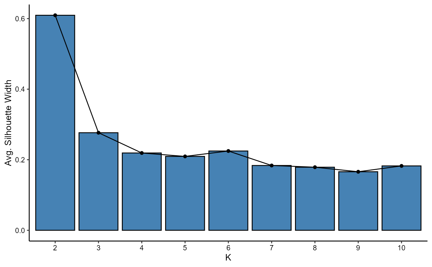

Figure 4.1 Average silhouette width plot.

… and the silhouette widths for every observation.

plotSilhouetteWidths(object, variable_set = "intensity", k = 2:10, ncol = 3)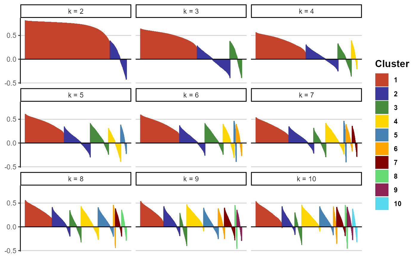

Figure 4.2 Silhouette width plot.

4.3 Add PAM cluster variables

Add the cluster variables of interest via addPamClusterVariables().

object <- addPamClusterVariables(object, variable_set = "intensity", k = c(4,5))

getClusterVariableNames(object, contains("pam"))

## [1] "pam_euclidean_k_4_(intensity)" "pam_euclidean_k_5_(intensity)"

5. Multiple clustering results

This example uses the variable set intensity defined in a similar fashion as shown in this [tutorial]. Since every cluster initiation gets its own slot clustering for as many variable sets as desired can coexist in the cypro object.

printAnalysisSummary(object, slots = "clustering")

## 
## --------------------------------------------------
## 
## Conducted analysis:
## 
## 
## 
## 
## |clustering |intensity |area |
## |:----------|:---------|:----|
## |hclust     |Yes       |No   |
## |kmeans     |Yes       |No   |
## |pam        |Yes       |No   |
## 
## 
## 
## --------------------------------------------------

object <- initiateHierarchicalClustering(object, variable_set = "area")

printAnalysisSummary(object, slots = "clustering")

## 
## --------------------------------------------------
## 
## Conducted analysis:
## 
## 
## 
## 
## |clustering |intensity |area |
## |:----------|:---------|:----|
## |hclust     |Yes       |Yes  |
## |kmeans     |Yes       |No   |
## |pam        |Yes       |No   |
## 
## 
## 
## --------------------------------------------------

6. Renaming cluster variables and cluster groups

To ensure unambiguous naming with respect to algorithm, variable set, methods etc. the initial clustering names are somewhat bulky. In addition to that are cluster named by number which is barely informative. In case you want to rename cluster variables or single cluster groups of a variable have a look at the tutorial about how to rename content in cypro.