1. Introduction
The amount of data generated by high throughput microscopy is immense. This can result in cypro objects containing hundreds of thousands of cells. Consider the example object below.
# load packages
library(cypro)
library(tidyverse)
library(patchwork)

object_original <- readRDS(file = "data/bids-week4-big.RDS")

object_original
## An object of class 'cypro'.
##
## Name: bids-week4
## Type: One Time Imaging
## Number of Cells: 86201
## Conditions: '5-fluorouracil', 'AG-1478', 'anisomycin', 'AZ258', 'caspase inhibitor (ZVAD)', 'cyclohexamide', 'DMSO', 'indirubin monoxime', 'mitomycin C', 'neomycin', 'okadaic acid', 'olomoucine', 'taxol' and 'tunicamycin'
## Cell Lines: 'MCF7'
## Well Plates: 'Week4_27481' and 'Week4_27801'
## Variable Sets: 'intensity'Even 86000 cells are enough for certain machine learning algorithms to surrender. For instance, Rs partitioning around medoids (PAM) implementation cluster::pam() does not work with more than 83.000 observations. Apart from computational efficiency you might want to focus on only subsets of cells, compute subcluster of a certain cluster etc. This is where you can make use of cypros subsetting functions:
subsetByCellId()subsetByCellLine()subsetByGroup()subsetByCondition()subsetByFilter()subsetByGroup()subsetByNumber()subsetByQuality()
They allow to conveniently split the data of your experiment into sub-cypro objects by a variety of aspects. On top of that the subsetting functions store the history of subsets in the sub-cypro objects. You can therefore always trace your analysis back to the original one.
printSubsetHistory(object = object_original)## Provided cypro object has not been subsetted yet.2. Subset by number
Having computational efficiency in mind you can reduce the number of cells by randomly selecting cells while forcing equal numbers of cells across specific groups - such as cell line and condition.
(If you are interested in analyzing proliferation and cell counts under certain conditions and treatments you should not use this function.)
# reduce the total number of cells to  ~ 50.000
object_reduced <-
  subsetByNumber(
    object = object_original,
    new_name = "bids-w4-red",
    across = "condition",
    n_total = 50000
    )

# equal number of cells across conditions
plotBarchart(object_original, variables = "condition", position = "stack") +
  coord_flip() +
  ggtitle("Original") +

plotBarchart(object_reduced, variables = "condition", position = "stack") +
  coord_flip() +
  ggtitle("Reduced")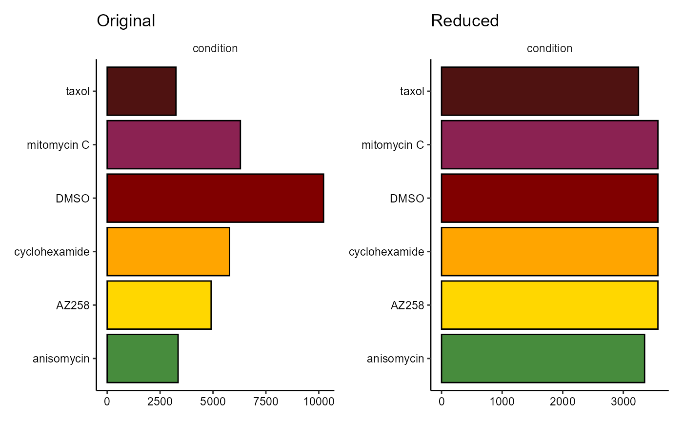
Figure 2.1 Adjustment of cell count as across was specified as ‘condition’
3. Subset by groups and conditions
You can create subsets according to all grouping variables your cypro object contains. (subsetByCellLine() and subsetByCondition() are wrapper around subsetByGroup().)
getGroupingVariableNames(object_reduced, verbose = F)output
## [1] "cell_line"        "condition"        "concentration"    "moa"
## [5] "well_plate_name"  "well_plate_index" "well"             "well_roi"
For instance, create subsets by wells if they share characteristics of interest.
# all wells
getGroupNames(object_reduced, grouping_variable = "well")
output
##  [1] "B10" "B11" "B2"  "B3"  "B4"  "B5"  "B6"  "B7"  "B8"  "B9"  "C10" "C11"
## [13] "C2"  "C3"  "C4"  "C5"  "C6"  "C7"  "C8"  "C9"  "D10" "D11" "D2"  "D3"
## [25] "D4"  "D5"  "D6"  "D7"  "D8"  "D9"  "E10" "E11" "E2"  "E3"  "E4"  "E5"
## [37] "E6"  "E7"  "E8"  "E9"  "F10" "F11" "F2"  "F3"  "F4"  "F5"  "F6"  "F7"
## [49] "F8"  "F9"  "G10" "G11" "G2"  "G3"  "G4"  "G5"  "G6"  "G7"  "G8"  "G9"
# b wells
b_wells <- getGroupNames(object_reduced, grouping_variable = "well", starts_with("B"))

b_wells
output
## [1] "B10" "B11" "B2" "B3" "B4" "B5" "B6" "B7" "B8" "B9"
object_bwells <-
  subsetByGroup(
    object = object_reduced,
    grouping_variable = "well",
    groups = b_wells
    )

object_bwells
output
## An object of class 'cypro'.
##
## Name: bids-w4-red_subset
## Type: One Time Imaging
## Number of Cells: 8060
## Conditions: 'anisomycin', 'cyclohexamide', 'DMSO' and 'taxol'
## Cell Lines: 'MCF7'
## Well Plates: 'Week4_27481' and 'Week4_27801'
## Variable Sets: 'intensity'
4. Subset by filter
Another option would be to create a subset in style of dplyr::filter() by filtering for cells that match certain requirements.
# remove obviuos outlier cells
object_normal_cells <-
  subsetByFilter(object_bwells, new_name = "normal-sized", AreaShape_Area < 20000 )

plotHistogram(object_bwells, variables = "AreaShape_Area") +
  ggtitle("Before subsetting") +

plotHistogram(object_normal_cells, variables = "AreaShape_Area") +
  ggtitle("After subsetting")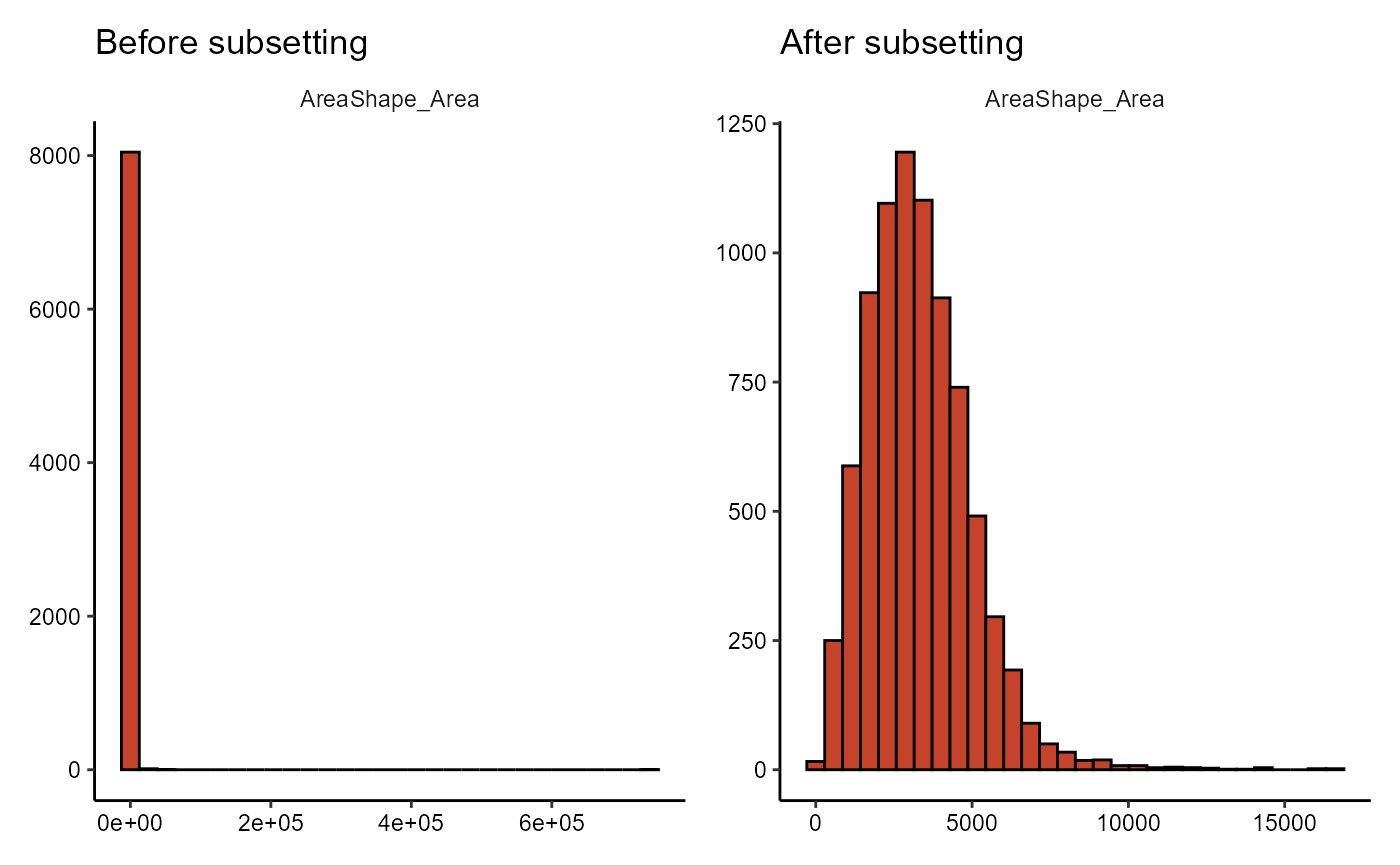
Figure 4.1 Difference in distribution before and after subsetting.
The function printSubsetHistory() keeps track of the subsetting.
printSubsetHistory(object_normal_cells)##
## First Subsetting:
##
## By: Number
## Method: n_total
## Weighted: FALSE
## Across: 'condition'
## Parent object: bids-week4
## New object: bids-w4-red
## Cells remaining: 49453
##
## --------------------------------------------------
##
## Second Subsetting:
##
## By: Group
## Grouping Name: 'well'
## Kept: 'B10', 'B11', 'B2', 'B3', 'B4', 'B5', 'B6', 'B7', 'B8' and 'B9'
## Parent object: bids-w4-red
## New object: bids-w4-red_subset
## Cells remaining: 8060
##
## --------------------------------------------------
##
## Third Subsetting:
##
## By: Filter
## Requirements:
## 1. AreaShape_Area<20000
## Parent object: bids-w4-red_subset
## New object: normal-sized
## Cells remaining: 8056