Prerequisites
Make sure to be familiar with the following tutorials before proceeding:
1. Introduction
After the use of designExperiment() the experiment design is now stored in the cypro-object called cypro_object_new. You can’t do any analysis and visualization with it yet as it does not contain any loaded data. To load data use the loadData*()- functions. There are two of them.
loadDataFile()is needed if the data is already present in one single file. This is often the case if CellProfiler has been used as the image processing software. This data table must contain variables giving information about the well, the region of interest (ROI) and - if the experiment design contains more than one well plate - about the well plate.loadDataFiles()is needed if the data is present in multiple files. This is the case if CellTracker has been used as the image processing software. In this case the information about the well-ROI and the well plate is conveyed by the names of the file (see below for more information).
2. Load multiple files
loadDataFiles() again opens a user interface. It is split in two parts.
2.1 Prepare data loading
The cypro package is very flexible regarding its input data. This flexibility comes with a small price: The name of important data variables such as x-coordinates, y-coordinates, Cell ID etc. must be single handedly denoted one by one. This is done during step 1 Prepare data loading.
2.2.1 Load template file
Here you upload an example file that is representative of all the other files that you will read in later on. Once the file is loaded you see the first six rows printed right below.
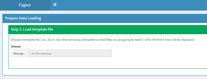
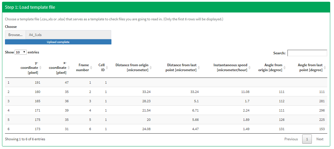
Figure 1 Load an example file.
The example file in this case is a track file derived from the image processing software Cell Tracker.
2.2.2 Denote identifier variables
As explained in the terminology article cyprorequires its input data to contain data variables that contain information about the cell id and the frame. In case of data files generated with CellTracker the variable names are obvious but they might change from software to software.
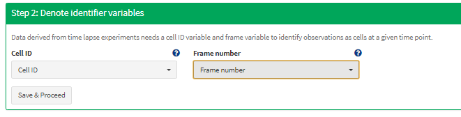
Figure 2 Tell cypro which columns refer to the cell id and the frame.
2.2.3 Denote module specific variables
Beyond the convenient possibility to read in huge amount of files according to specific experiment designs cypro offers a variety of analysis functionalities. Step 3: Denote module specific variables is about telling cypro where to get the required information as well as which modules it is supposed to use. Some of them require specific data variables (needed variables) based on which other variables are computed (computable variables). Every select input option is provided with a blue question mark which displays information about the variable to be denoted.
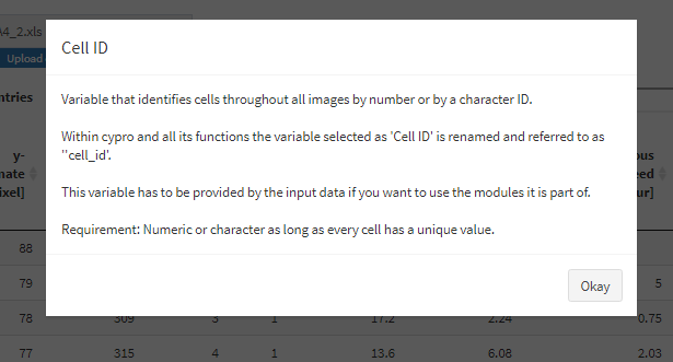
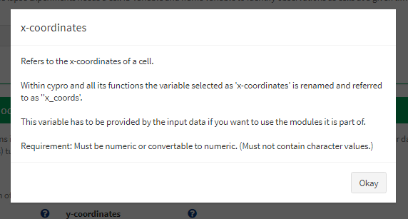
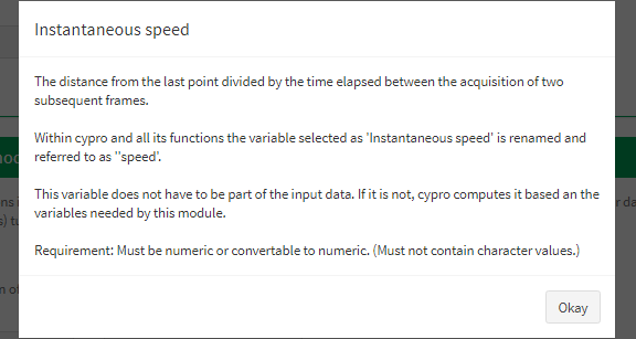
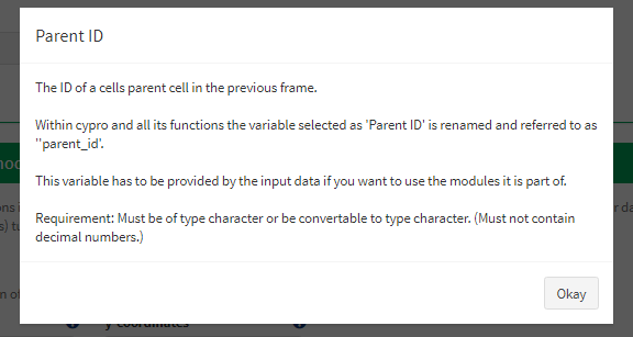
Figure 3 Example variable descriptions.
For instance, the migration module needs information about x- and y-coordinates. If not specified additionally data variables such as Distance from origin or Instantaneous speed can be computed. While basically every image processing software outputs x- and y-coordinates of the tracked cells information about cell splits are not part of every software output. If your data files do not contain needed variables for a certain module make sure to ‘turn off’ the module with the slider below it. In this case the CellTracker files do not contain mitosis related data. Therefore we won’t be able to use the mitosis module.
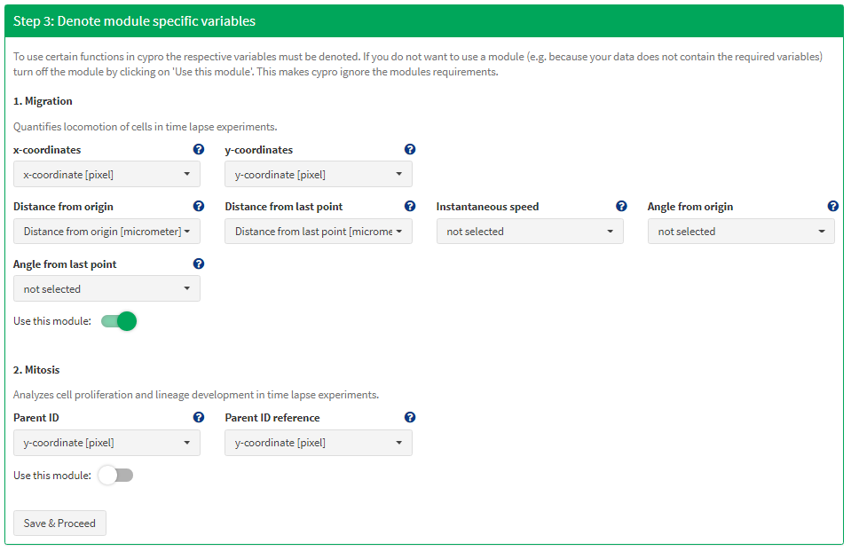
Figure 4 Tell cypro where to look for needed information.
2.2.4 Denote additional variables
Every additional data variable that is unknown to cypro but contains information you want to include in downstream analysis steps such as clustering and correlation can be denoted here. CellTracker does not offer any additional variables apart from those already integrated in our migration module.
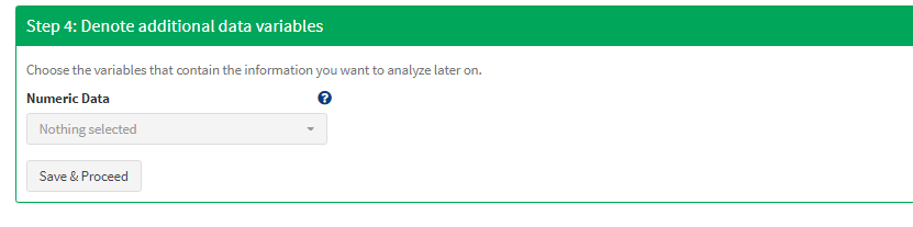
Figure 5 No data variables remain to be selected additionally.
In case of output files from CellProfiler it could look somewhat like this.
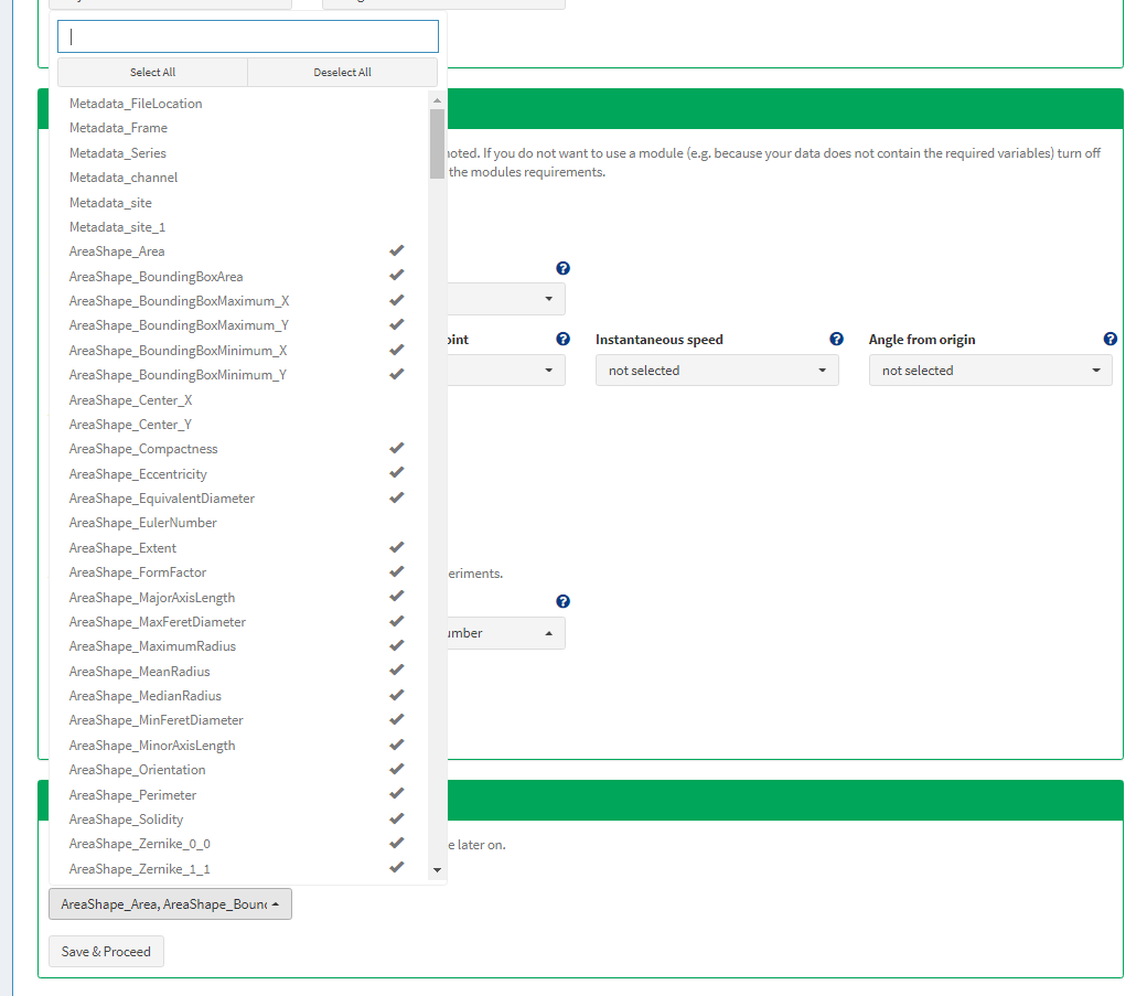
Figure 6 Tell cypro which addtional variables you want to analyze later on.
Note: Data variables denoted in Step 3 Denote module variables can be used for correlation and clustering, too! Step 4 Denote additional variables simply lets you keep data variables that do not have an inherent meaning to cypro while simultaneously lets you discard variables you won’t be interested in later on.
2.2.5 Last check
Every denoted variable name is saved as such. Based on the input from step 2, step 3, and step 4 the final data.frame as shown in Figure 7 is what cypro expects all files you are about to read in to look like. (The order of the data variables does not matter. However, missing data variables will result in an error during the reading process. See below.)
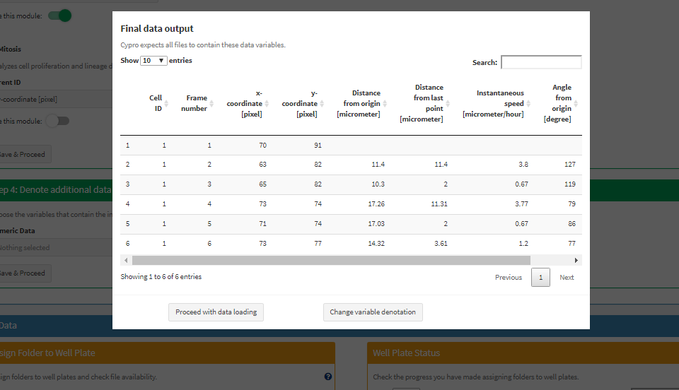
Figure 7 Double check that the data.frame cypro expects contains all information you need later on.
2.3 Load data
Once cypro knows what to expect you assign a folder to each well plate that you’ve previously designed in designExperiment(). cypro will then skim the folder and all its subfolders for data files that match the well-image names.
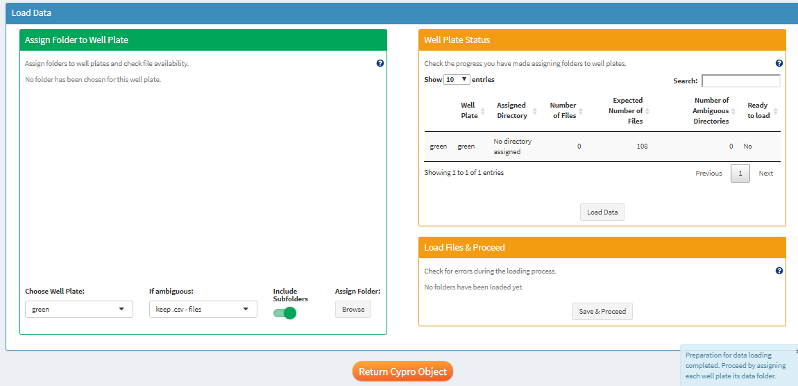
Figure 8 No folders have been assigned yet.
It takes the folder (here represented by ‘~/’) you’ve chosen and skims its content for files that end according to the following syntax:
- ~/…’Well’_‘ImageIndex’.’filetype’
Valid examples would be:
- ~/A1_1.xls
- ~/this_is_a_valid_filename_G3_2.xlsx
- ~/hidden/in/subfolders/H2_2.csv
Invalid examples:
- ~/A1-1.csv (does not use _ as a separator between well and image)
- ~/does_not_end_A1_1_accordingly.xls (the file name does not end with the well-image pattern)
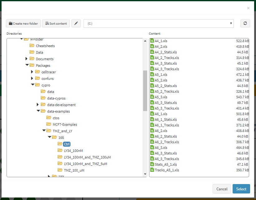
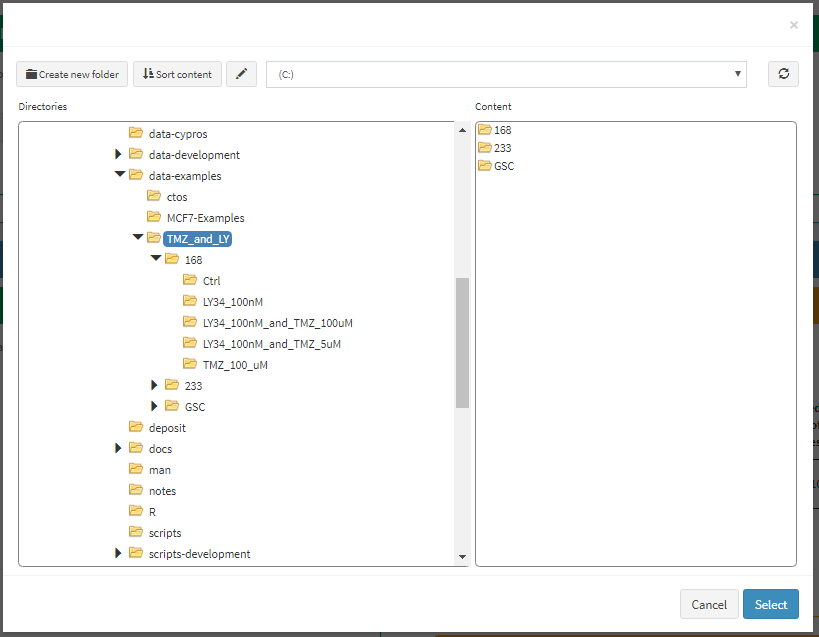
Figure 9 Pick the main folder that contains the data files of the respective well plate.
Note: Although the actual files are stored in subfolders choosing the folder TMZ_and_LY as the folder that contains all files for the respective well plate is the way to go as cypro looks into the subfolders as well.
Once the folder is assigned cypro evaluates by well how many of the expected files were found and indicates that by plotting the well plate colored according to the file availability (Figure 10).
For instance, the well plate designed here contained information for wells in rows A, D, E and H and columns 1-9. The input box ‘Images per Well’ was set to 3. cypro therefore expects to find three files for every well named according to the syntax mentioned above. Depending on the number of matching files found one of the four colors appears:
Green: All files were found for that well.
Yellow: Some files were found for that well.
Red: No files were found for that well.
Blue: More than the expected number of files were found. This can happen if files are stored in subfolders and accidentally were named equally.
For instance files ~/subfolder1/A1_1.csv and ~/subfolder2/A1_1.csv would result in well A1 appearing blue.
Note: Figure 9 shows the content of folder ~/168/Ctrl/. It contains several files with the well-image pattern A4_2. However, only one of the file names is valid which is why the evaluation plot in Figure 10 does not indicate that there are any ambiguous files. On the other hand there are several files that end with the well image pattern A5_1. Although the files are prefixed differently cypro does not recognize the difference as it considers all files that end with a well-image pattern as valid. The input for well image A5_1 is ambiguous. Ambiguous files need to be either removed or renamed.
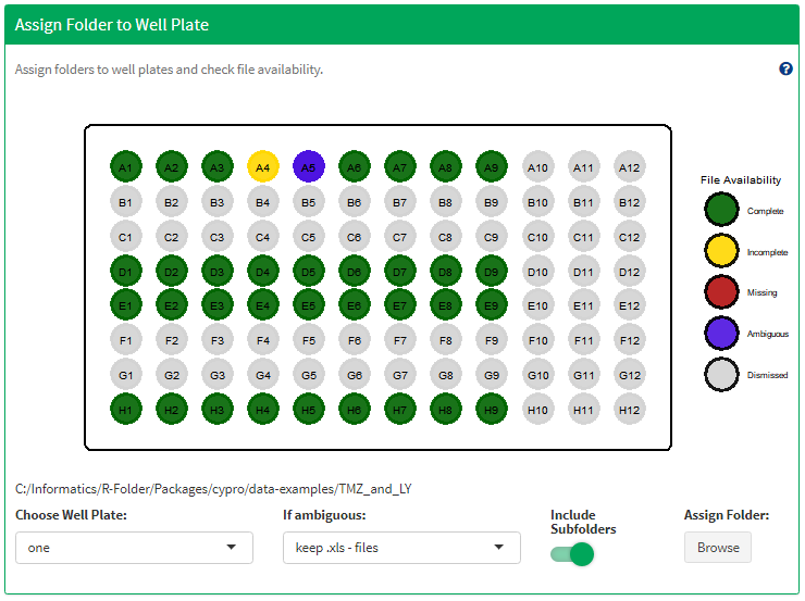
Figure 10 Wells that were dismissid in designExperiment() are ignored and always displayd in grey.
In case of missing files the well plate plotted could look like this. (A well plate from a different experiment design.)
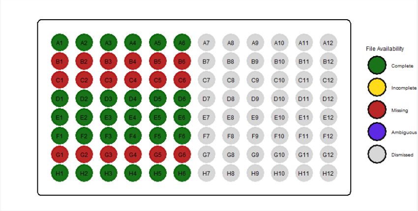
Figure 11 If no files were found the wells are displayed in red.
Missing and incomplete wells do not prevent you from loading the data. If you realize that some files are missing, check for possible naming issues, correct what needs to be corrected and then assign the folder again. The file availability is reevaluated and colors should change accordingly. Once all well plates have a folder assigned to them and no ambiguous files were found the box ‘Well Plate Status’ turns green indicating that the data is ready to be loaded.
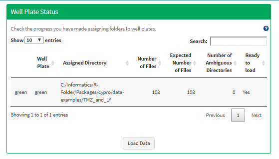
Figure 12 A green ‘Well Plate Status’ box indicates that the data files are ready to be loaded.
After clicking on ‘Load Data’ a progress bar is going to appear in the lower right corner indicating the loading progress. While being loaded all files are checked to match the requirements set up during the variable denotation. If any errors occur during the loading process they are presented in the box ‘Load Files & Proceed’ in combination with the error message returned.
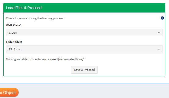
Figure 13 If errors occured while loading some files they are listed here.
Again, you can choose to ignore failed files and simply proceed without them by clicking on ‘Save & Proceed’ and then on ‘Return Cypro Object’. If possible you can fix the reason that prevented cypro from reading the file successfully and click on ‘Load Data’ again.
3. Load one file
The way loadDataFile() works is very similar to the way loadDataFiles() works. There are two differences:
Instead of uploading a template file you immediately upload the file that contains all the data.
Before denoting the module specific variables you need to denote the ones that contain the information about the well plate, well and ROI.
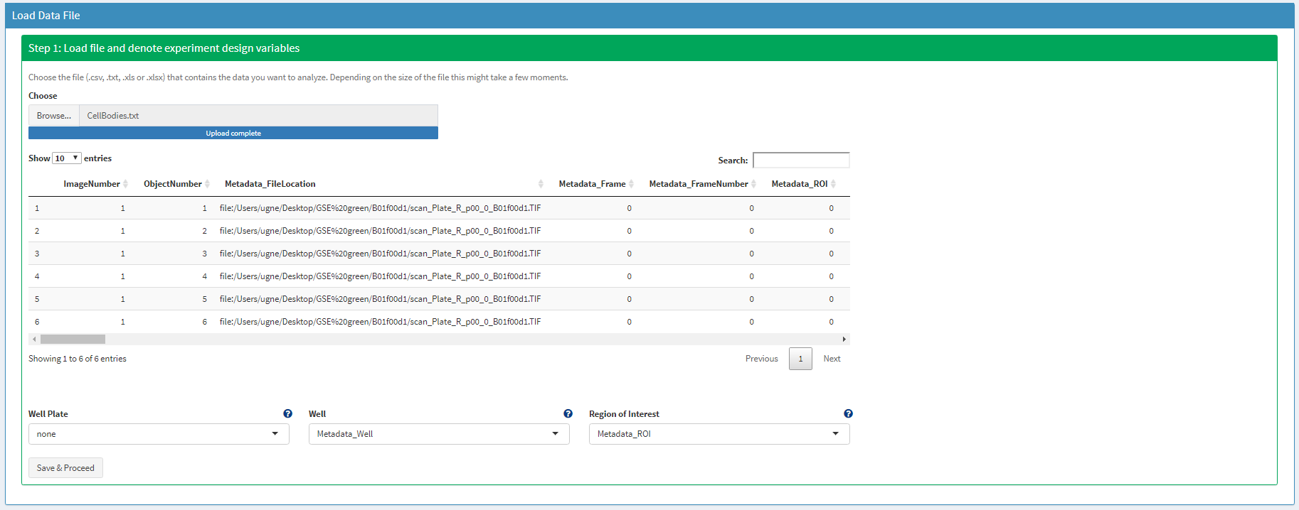
Figure 14 The interface of loadDataFile() looks slightly different.
These experiment design variables are then checked for validity. If they can be used to match the data to the experiment design you can proceed with denoting the module specific variables as described above and eventually return the cypro-object that now contains the data.