Correlation • cypro

Prerequisites

Make sure to be familiar with the following tutorials before proceeding:

Variable Sets

1. Introduction

In a similar fashion to clustering correlation analysis in cypro is conducted on the base of variable sets.

# load packages
library(cypro)

# load object from broad institute compound profiling experiment week 4
# contains one time imaging data
object <- readRDS(file = "data/bids-week4.RDS")

# load object that contains tracking data 
object_tracks <- readRDS(file = "data/example-tracks.RDS")

2 Initiate correlation

We introduced variable sets with examples in which they contained only variables of one kind (e.g. shape or intensity). However, variable sets can contain as many variables of as many different kinds as desired.

granularity_vars <- getStatVariableNames(object, starts_with("Granularity"))

intensity_vars <- getVariableSet(object, "intensity")

object <- addVariableSet(object, variable_names = c(granularity_vars, intensity_vars), set_name = "gran_intensity")

Once the variable set is defined you can set up the correlation analysis with initiateCorrelation().

object <- initiateCorrelation(object, variable_set = "gran_intensity")

3. Computation

cypro allows to compute correlation without regarding grouping options or in a comparative manner. The function correlateAll()takes all variables in the defined variables set and calculates correlation as well as belonging p-values.

object <- correlateAll(object, variable_set = "gran_intensity", method_corr = "pearson")

The function correlateAcross() allows to additionally specify grouping variables according to which data is split before calculating correlation. This comes in very handy when to investigate in how far the relation between variables changes across cell lines or cluster or in how far the relation is disturb under certain conditions.

object <- correlateAcross(object, variable_set = "gran_intensity", across = c("condition"))

As in clustering all results are stored separately in the cypro object and can be plotted and extracted as well as they can expanded with computations for grouping variables that are added after initiateCorrelation(). For instance, if you have added a new clustering variable via addKmeansClusterVariables() and you now want to compute the correlation for all variables across these clustering results just use correlateAcross()again and specify the clustering name with the argument across.

# add cluster variable 
object <- addKmeansClusterVariables(object, variable_set = "area", k = 4, method_kmeans = "Lloyd")

# obtain respective name
getClusterVariableNames(object, contains(c("kmeans", "area", "4")))

# add another comparative correlation 
object <- correlateAcross(object, variable_set = "gran_intensity", across = "kmeans_Lloyd_k_4_(area)")

4. Visualize

The function plotCorrplot() comes with a lot of options to visualize the relation between variables. You find a detailed description of how it works by typing ?plotCorrplot in your R console. Below are some examples of how to visualize your results. Note: plotCorrplots() returns a ggplot. This has the advantage that it is very flexible and can be adjusted even after plotting. A drawback is, that geometric objects like circles or rectangulars have to be adjusted in size manually to be aesthetically pleasing.

As variable names occupy a lot of space in correlation plots we use renameStatsDfWith() or renameTracksDfWith() to shorten the stat variable names. The tutorial about renaming elaborates on how to do that.

object <- 
  renameTracksDfWith(
    object = object,
    # remove redundant pre- and suffixes ...
    .fn = ~ stringr::str_remove_all(.x, pattern = "^Intensity_|_Actin"),
    # ... of variables that start with either of both names
    .cols = starts_with(c("Intensity", "Granularity")) 
    )

4.1 Correlation plots

plotCorrplot() without specifying argument across visualizes the correlation values of variables irrespective of cell grouping.

plotCorrplot(object, variable_set = "gran_intensity", plot_type = "lower", shape = "circle", shape_size = 2)

plotCorrplot(object, variable_set = "gran_intensity", plot_type = "complete")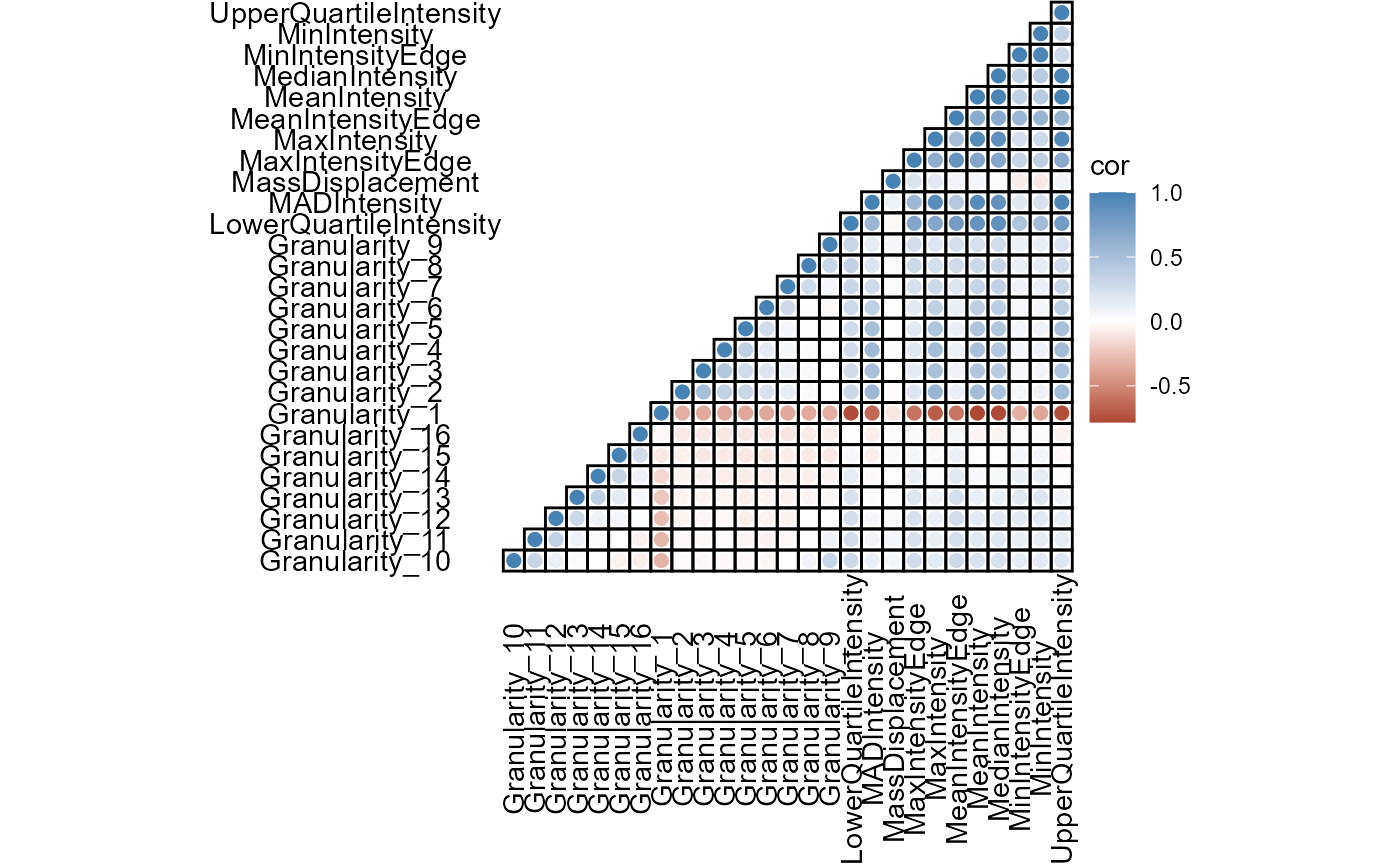

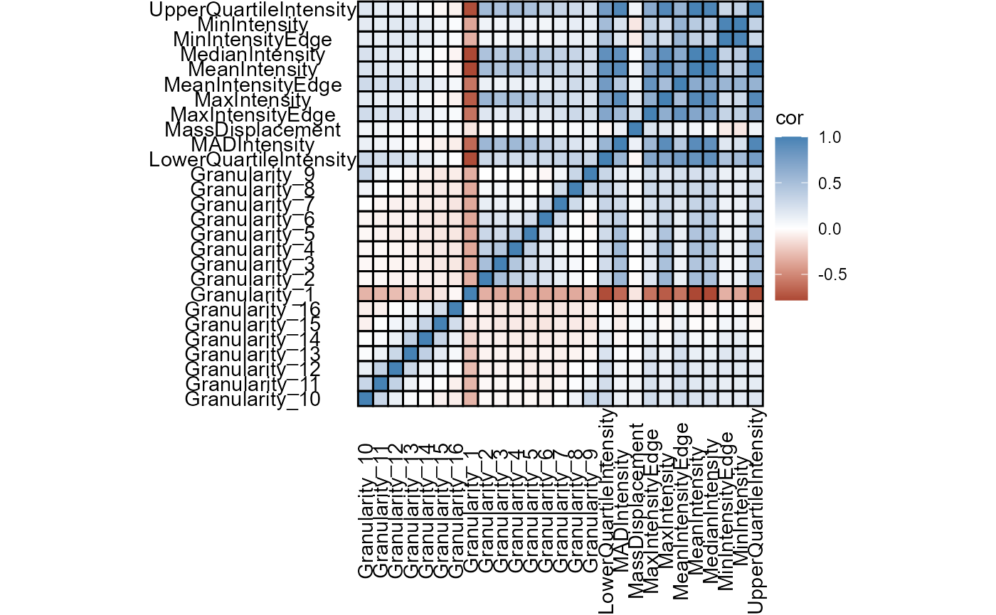
Figure 4.1 Basic correlation plots come in a variety of shapes and aesthetics.

4.2 Correlation across groups

Using argument across allows to investigate changes in variables relations in different groups. across_subset allows to specify the the groups of interest.

# obtain valid input options for across_subset
conditions <- getConditions(object)

plotCorrplot(
  object = object,
  variable_set = "gran_intensity",
  plot_type = "complete",
  shape = "rect",
  shape_size = 1.5,
  across = "condition",
  across_subset = c("DMSO", "taxol", "AZ258"),
  nrow = 1
  ) +
  labelsXremove() + 
  labelsYremove()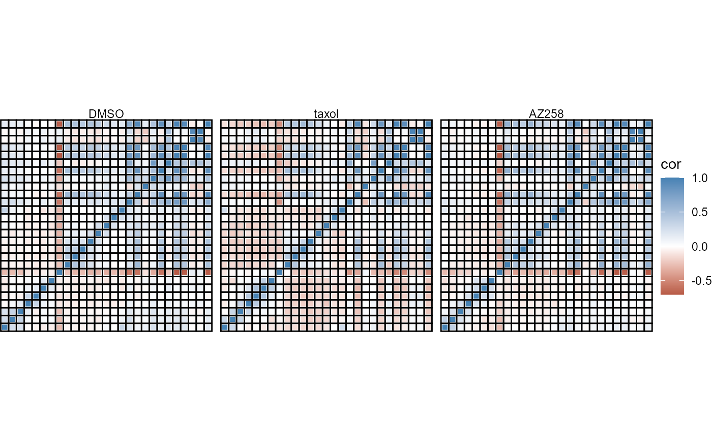

Figure 4.2 Comparative correlation plots.

4.3 Significance levels

By specifying argument signif_level you can set a maximum p-value threshold for the correlation. All correlations with a p-value above that threshold are crossed out.

plotCorrplot(
  object = object,
  variable_set = "gran_intensity",
  plot_type = "complete",
  shape = "rect",
  shape_size = 1.5,
  signif_level = 0.01,
  across = "condition",
  across_subset = c("DMSO", "taxol", "AZ258"), 
  nrow = 1
  ) + 
  labelsXremove() + 
  labelsYremove()

Figure 4.3 Integrate significance thresholds.

5. Extraction

Correlation results are stored in the @analysis-slot under $correlation. Every correlation for every variable set is stored in a specific S4-object as programmed in the package confuns called corr_conv. Use the function getCorrObject() to extract the S4-objects containing all data needed including correlation matrices and p-values.